Materials
Data
This lesson uses data on arrests around athletics venues in Cleveland, Ohio to address questions of the effects of sporting events on the frequency, timing, and type of crimes.
Menaker, BE, DA McGranahan & RD Sheptak Jr. 2019. Game Day Alters Crime Pattern in the Vicinity of Sport Venues in Cleveland, OH. Journal of Sport Safety and Security 4(1):art.1
Script
Video lecture
Walking through the script
Load packages and data
pacman::p_load(tidyverse)
clev_d <- read_csv("./data/AllClevelandCrimeData.csv")
clev_d
## # A tibble: 241 x 11
## Address Date Time ReportedCharge GeneralCharge ChargeType GameDay Venue
## <fct> <fct> <fct> <fct> <fct> <fct> <int> <fct>
## 1 "1 LAK… "1/1… 11:47 " DOMESTIC VI… DOMESTIC VIO… DOMESTIC … 0 FE
## 2 "LAKES… "2/1… 10:20 " DOMESTIC VI… DOMESTIC VIO… DOMESTIC … 0 FE
## 3 "ONTAR… "1/2… 14:00 " DOMESTIC VI… DOMESTIC VIO… DOMESTIC … 0 FE
## 4 "100 A… "8/1… 22:20 "DOMESTIC VIO… DOMESTIC VIO… DOMESTIC … 1 FE
## 5 "300 E… "5/4… 12:51 " DOMESTIC VI… DOMESTIC VIO… DOMESTIC … 0 FE
## 6 "LAKES… "9/1… 12:48 " DOMESTIC VI… DOMESTIC VIO… DOMESTIC … 0 FE
## 7 "727 B… " 2/… 2:00 " 3 DOMESTIC … DOMESTIC VIO… DOMESTIC … 1 GP
## 8 "900 C… "2/2… 2:00 " 3 DOMESTIC … DOMESTIC VIO… DOMESTIC … 1 GP
## 9 " ONTA… "10/… 13:30 " 13 DOMESTIC… DOMESTIC VIO… DOMESTIC … 0 GP
## 10 "ONTAR… " 9/… 2:00 " 13 DOMESTIC… DOMESTIC VIO… DOMESTIC … 0 GP
## # … with 231 more rows, and 3 more variables: AirTemp <int>, Day <fct>,
## # Event <fct>How many types of crimes occur in Cleveland?
nlevels(clev_d$ReportedCharge)## [1] 96Wow, that’s a lot, what are they?
levels(clev_d$ReportedCharge)## [1] " 13 ASSAULT"
## [2] " 13 ASSAULT - SIMPLE"
## [3] " 13 CRIMINAL TRESPASSING W/O PRIVILEGE TO DO SO:"
## [4] " 13 DOMESTIC VIOLENCE"
## [5] " 13 GIVING FALSE INFORMATION TO ENFORCEMENT AGENTS"
## [6] " 13 MENACING"
## [7] " 13 MOTOR VEHICLE TRESPASS"
## [8] " 13 POSSESSING CRIMINAL TOOLS"
## [9] " 13 RESISTING ARREST"
## [10] " 13 ROBBERY-FIREARM-HIGHWAY(STREET"
## [11] " 13 ROBBERY-FIREARM-MISCELLANEOUS"
## [12] " 13 ROBBERY-KNIFE-MISCELLANEOUS"
## [13] " 13 ROBBERY-STRONG ARM-HIGHWAY"
## [14] " 13 ROBBERY-STRONG ARM-RESIDENCE"
## [15] " 3 AGGRAVATED MURDER-NON NEGLIGENCE"
## [16] " 3 ASSAULT"
## [17] " 3 ASSAULT-RECKLESS-HANDS/FISTS/FEET-SERIOUS HARM )"
## [18] " 3 ASSAULT - SIMPLE"
## [19] " 3 ASSAULT ON POL OFF - SIMPLE ASSAULT"
## [20] " 3 CONTRIB TO UNRULINESS OR DELINQUENCY OF A CHILD"
## [21] " 3 CRIMINAL TOOLS"
## [22] " 3 CRIMINAL TRESPASS"
## [23] " 3 CRIMINAL TRESPASSING -KNOWINGLY ENTER/REMAIN"
## [24] " 3 CRIMINAL TRESPASSING W/O PRIVILEGE TO DO SO:"
## [25] " 3 DOMESTIC VIOLENCE"
## [26] " 3 FEL ASSLT - POLICE OFF - FIREARM"
## [27] " 3 FEL ASSLT - POLICE OFF - HANDS/FISTS/FEET"
## [28] " 3 FELONIOUS ASSAULT - FIREARM"
## [29] " 3 FELONIOUS ASSAULT - HANDS"
## [30] " 3 FELONIOUS ASSAULT - KNIFE OR CUTTING INSTRUMENT"
## [31] " 3 FELONIOUS ASSAULT - OTHER DANGEROUS WEAPON"
## [32] " 3 FELONY - FLEEING AND ELUDING"
## [33] " 3 MENACING"
## [34] " 3 MOTOR VEHICLE TRESPASS"
## [35] " 3 OBSTRUCTING JUSTICE"
## [36] " 3 OBSTRUCTING OFFICIAL BUSINESS"
## [37] " 3 POSSESSNG CERTAIN WEAPONS AT OR ABOUT PUBLIC PLACE"
## [38] " 3 PURCHASE CONSUMPTN OR POSSESSN BY MINOR:MISREPRESN"
## [39] " 3 RESISTING ARREST"
## [40] " 3 ROBBERY-FIREARM-GAS OR SERVICE STATION"
## [41] " 3 ROBBERY-FIREARM-HIGHWAY(STREET"
## [42] " 3 ROBBERY-FIREARM-MISCELLANEOUS"
## [43] " 3 ROBBERY-ODW-MISCELLANEOUS"
## [44] " 3 ROBBERY-STRONG ARM-GAS OR SERVICE STATION"
## [45] " 3 ROBBERY-STRONG ARM-HIGHWAY"
## [46] " 3 ROBBERY-STRONG ARM-MISCELLANEOUS"
## [47] " 3 STOPPING OR SLOW SPEED; POSTED MINIMUM"
## [48] " 3 TELEPHONE HARASSMENT"
## [49] " 5 AGGRAVATED MENACING"
## [50] " 5 ASSAULT"
## [51] " 5 ENDANGERING CHILDREN"
## [52] " 5 POSSESSING CRIMINAL TOOLS"
## [53] " AGGRAVATED MENACING"
## [54] " AGGRAVATED RIOT"
## [55] " ASSAULT"
## [56] " ASSAULT-RECKLESS-HANDS/FISTS/FEET-SERIOUS HARM )"
## [57] " ASSAULT ON POL OFF - SIMPLE ASSAULT"
## [58] " CRIMINAL TRESPASS"
## [59] " CRIMINAL TRESPASSING -KNOWINGLY ENTER/REMAIN"
## [60] " CRIMINAL TRESPASSING W/O PRIVILEGE TO DO SO:"
## [61] " DOMESTIC VIOLENCE"
## [62] " ENDANGERING CHILDREN"
## [63] " FAIL TO PROVIDE FOR FUNCTIONALLY IMPAIRED PERSON"
## [64] " FELONIOUS ASSAULT - HANDS"
## [65] " FELONIOUS ASSAULT - KNIFE OR CUTTING INSTRUMENT"
## [66] " FELONIOUS ASSAULT - OTHER DANGEROUS WEAPON"
## [67] " GROSS SEXUAL IMPOSITION"
## [68] " HARASSMENT BY INMATE"
## [69] " MENACING"
## [70] " MENACING BY STALKING"
## [71] " MOTOR VEHICLE TRESPASS"
## [72] " OBSTRUCTING OFFICIAL BUSINESS"
## [73] " PEDDLING ON PRIVATE PROPERTY:PERMIT"
## [74] " PURCHASE CONSUMPTN OR POSSESSN BY MINOR:MISREPRESN"
## [75] " RESISTING ARREST"
## [76] " RIOT"
## [77] " ROBBERY-FIREARM-MISCELLANEOUS"
## [78] " ROBBERY-ODW-MISCELLANEOUS"
## [79] " ROBBERY-STRONG ARM-HIGHWAY"
## [80] " SEXUAL IMPOSITION"
## [81] " TELEPHONE HARASSMENT"
## [82] " TEMPORARY PROTECTION ORDER"
## [83] "13 DOMESTIC VIOLENCE"
## [84] "13 TELEPHONE HARASSMENT"
## [85] "3 ASSAULT"
## [86] "3 KIDNAPPING"
## [87] "3 MENACING"
## [88] "3 RESISTING ARREST"
## [89] "3 SEXUAL IMPOSITION"
## [90] "ASSAULT"
## [91] "ASSAULT - FEETS ETC"
## [92] "ASSAULT ON POL OFF - SIMPLE ASSAULT"
## [93] "DOMESTIC VIOLENCE"
## [94] "MOTOR VEHICLE TRESPASS"
## [95] "RAPE"
## [96] "RESISTING ARREST"There is a lot of similarity among these specific charges. Let’s view a column of more general designations:
levels(clev_d$GeneralCharge)## [1] " AGGRAVATED MURDER" "ASSAULT"
## [3] "DOMESTIC VIOLENCE" "ENDANGERING CHILDREN"
## [5] "GROSS SEXUAL IMPOSITION" "HARASSMENT"
## [7] "KIDNAPPING" "MENACING"
## [9] "MINOR ALCOHOL" "OBSTRUCTION"
## [11] "OTHER" "PROPERTY"
## [13] "PROPERTY " "RAPE"
## [15] "RESISTING ARREST" "RIOT"
## [17] "ROBBERY" "SEXUAL IMPOSITION"
## [19] "WEAPON"Bar plots for counts
We can use a bar plot to see how many of each charge type occurs in the dataset.
Note that when stat = 'count', geom_bar knows automatically that the Y axis will be the count of each level in the categorical vector assigned to X:1
ggplot(clev_d)  +
  geom_bar(aes(x=GeneralCharge),
           stat="count")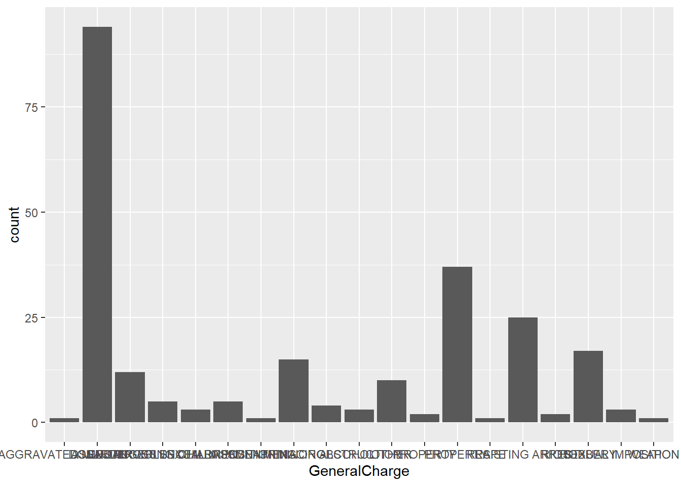
The utility of this graph is obvious, but it is far too messy at this point to be useful.
The following steps apply some clean-up.
Note here the use of the reorder function, to arrange the order of the X axis by the number of charges in each type, rather than alphabetically:
charges_gg <-
  ggplot(clev_d)  + theme_bw(14) +
    geom_bar(aes(x=reorder(GeneralCharge,
                           GeneralCharge,
                           function(x)-length(x))),
             stat="count")
charges_gg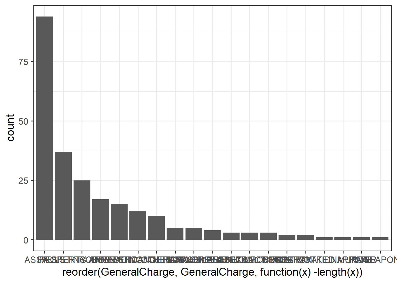
Here we add informative labels:
charges_gg <- charges_gg +
                labs(x="Charge type",
                     y="Frequency of incidents")
charges_gg
Now some more power-user tricks in ggplot.
One can use theme() to tweak components of the plot that aren’t directly manipulated by aes(), scale_*, or geom_* commands.
There are dozens of theme elements; see ?theme.
Many are grouped into just a few elements_.
Here we use element_text to modify the X axis text (tick mark identifiers) and element_blank as a quick way to turn off or remove another component, the vertical lines that help guide a viewer’s eye to the axis value (unnecessary when there’s a bar coming stright up out of the value!).
angle= rotates the labels a given number of degrees, and hjust= controls the horizontal alignment of the label text: \(0\) for full left, \(0.5\) for centered, and \(1\) for right alignment:
charges_gg +
  theme(axis.text.x=element_text(angle=45,
                                 hjust=1,
                                 color = "black"),
        panel.grid.major.x = element_blank())
Clearly a lot of charges aren’t very frequent.
It would make the graph a lot less busy if they could just be assigned to an ‘’other’’ category.
The ChargeType column does this already:2
ggplot(clev_d)  + theme_bw(14) +
  geom_bar(aes(x=reorder(ChargeType,
                         ChargeType,
                         function(x)-length(x))),
           stat="count") +
  labs(x="Charge type",
       y="Frequency of incidents") +
  theme(axis.text.x=element_text(angle=45,
                                 hjust=1,
                                 color = "black"),
        panel.grid.major.x = element_blank() )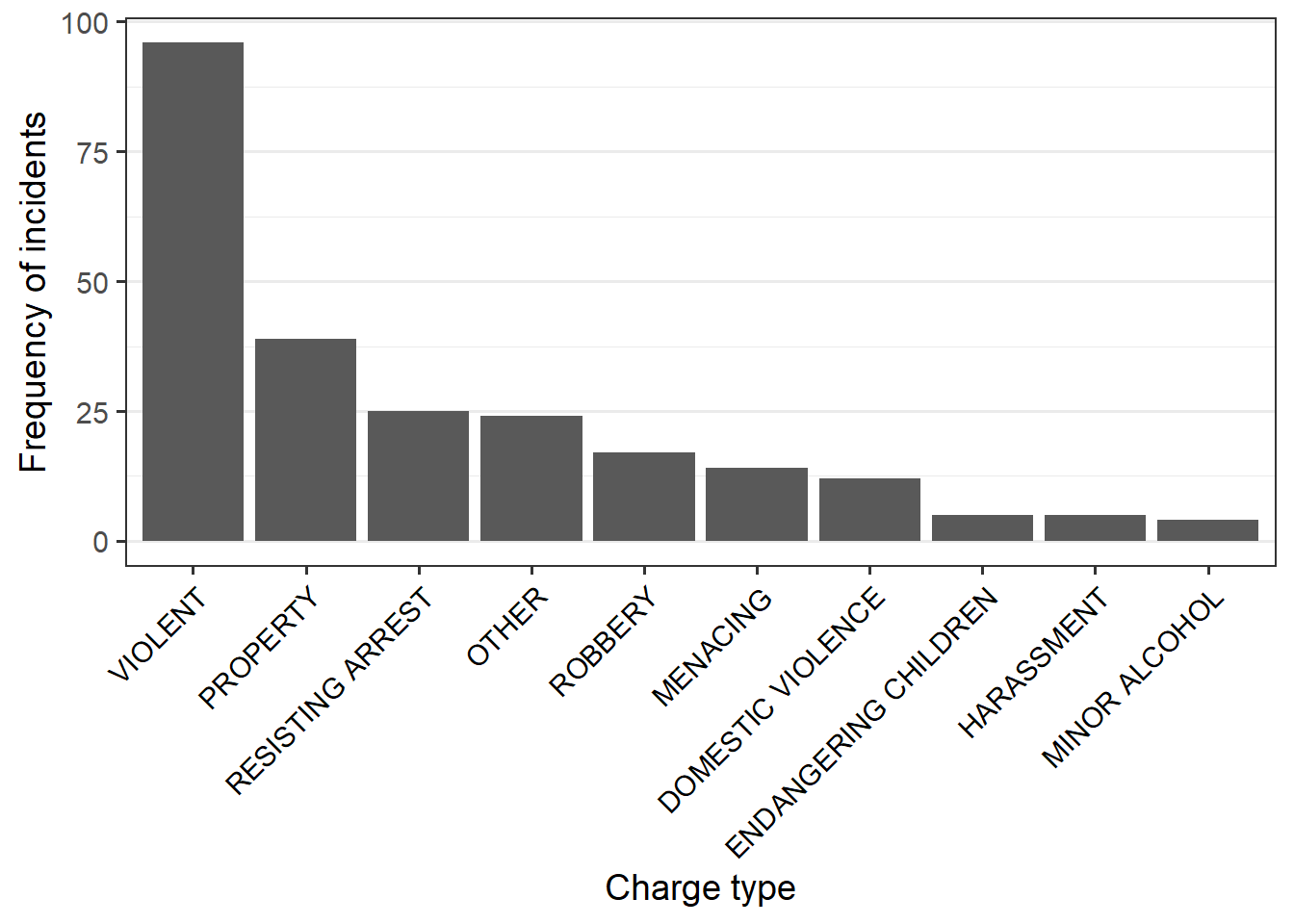
Game day vs. non-game day
To get back to the the research question: Which types of crame vary by game day?
Previously, we had used length(<vector>) to count up the number of observations in a vector.
But in this dplyr pipe we can use this easy little function n():
clev_d %>%
  group_by(ChargeType, GameDay) %>%
      summarize(charges=n()) %>%
pander::pander()| ChargeType | GameDay | charges |
|---|---|---|
| DOMESTIC VIOLENCE | 0 | 8 |
| DOMESTIC VIOLENCE | 1 | 4 |
| ENDANGERING CHILDREN | 1 | 5 |
| HARASSMENT | 0 | 2 |
| HARASSMENT | 1 | 3 |
| MENACING | 0 | 11 |
| MENACING | 1 | 3 |
| MINOR ALCOHOL | 1 | 4 |
| OTHER | 0 | 12 |
| OTHER | 1 | 12 |
| PROPERTY | 0 | 18 |
| PROPERTY | 1 | 21 |
| RESISTING ARREST | 0 | 2 |
| RESISTING ARREST | 1 | 23 |
| ROBBERY | 0 | 6 |
| ROBBERY | 1 | 11 |
| VIOLENT | 0 | 27 |
| VIOLENT | 1 | 69 |
A few things pop out:
- Arrests for some crimes only occur on game days, e.g. Minors in possession of alcohol, Endangering children.
- Frequency of some crimes goes down on game days, e.g. Domestic violence
- Other crimes seem to increase on game days.
Let’s add game day as a conditioning variable in our graph, using fill= to make what is known as a stacked bar graph:
  ggplot(clev_d) + theme_bw(14) +
    geom_bar(aes(x=reorder(ChargeType,
                           ChargeType,
                           function(x)-length(x)),
                 fill=factor(GameDay)),
             stat="count") +
    labs(x="Charge type",
         y="Frequency of incidents") +
    theme(axis.text.x=element_text(angle=45, hjust=1, color = "black"),
          panel.grid.major.x = element_blank(),
          legend.position=c(0.75,0.8),
          legend.key.width=unit(0.25, "in")) +
    scale_fill_brewer(palette="Set1",
                      name="Game day?",
labels=c("No","Yes")) 
From here, we can focus on the three most frequent charge types.
Note the column %in% c(..) construction to filter by multiple levels:
gd_charges <- clev_d %>%
                filter(ChargeType %in% c("VIOLENT",
                                       "RESISTING ARREST",
                                       "PROPERTY"))
 nlevels(gd_charges$ChargeType)
## [1] 10Note how even though we have filtered the ChargeType column to just the rows that match these three levels, as a factor vector class, the column still carries the original information about the levels in the column.
This is a quirk of factor vectors, and a reason to use character vector types.
However, it doesn’t often create actual problems.
But if it does, you can use droplevels to clear out unused levels from the vector:
gd_charges <- gd_charges %>%
               mutate(ChargeType = droplevels(ChargeType))
nlevels(gd_charges$ChargeType)
## [1] 3levels(gd_charges$ChargeType)## [1] "PROPERTY" "RESISTING ARREST" "VIOLENT"Stop the shouting!
Another aesthetic tweak would be to convert the ALL CAPS from the Cleveland Police data into something less shouty with tolower:
gd_charges <- mutate(gd_charges,
                      ChargeType = tolower(ChargeType) )
str(gd_charges$ChargeType)
## chr [1:160] "property" "property" "property" "property" "property" ...Note that this converts to a character vector.
Now view our cleaned-up, ready-to-publish graph:
  ggplot(gd_charges) + theme_bw(16) +
    geom_bar(aes(x=reorder(ChargeType,
                           ChargeType,
                           function(x)-length(x)),
                 fill=factor(GameDay)),
             stat="count",
             position = "dodge") +
    labs(x="Charge type",
         y="Frequency of incidents") +
    theme(axis.text.x=element_text(angle=45,
                                   hjust=1,
                                   color = "black"),
          panel.grid.major.x = element_blank(),
          legend.position=c(0.75,0.8),
          legend.key.width=unit(0.25, "in")) +
    scale_fill_brewer(palette="Set1",
                      name="Game day?",
labels=c("No","Yes")) 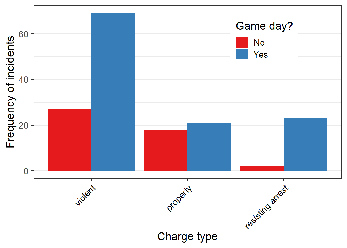
Time series
Data representing time are so different than other data types that several date and/or time specific object classes exist in the \({\bf\textsf{R}}\) landscape. On one hand, these object classes are notoriously challenging to work with. On the other hand, they carry a crazy amount of information that we can access in myriad ways. Indeed, it is this large amount of information that makes these objects so challenging, and the large amount of information is exactly why it is so valuable for data wranglers to learn how to use them.
\({\bf\textsf{R}}\) has several date/time object classes.
Because most of the tidyverse is compatible with one in particular, POSIXct, that’s what we’ll use here.
Create a timestamp
First we will create a timestamp. Anyone who uses data from electronic dataloggers is probably familiar with timestamps: a column that records when each row of data was collected or written to the file.
In this case, our data come from the CPD with one column for the date of the arrest, and another column for the time of day:
gd_charges %>%
  select(Date, Time)
## # A tibble: 160 x 2
## Date Time
## <fct> <fct>
## 1 10/13/2013 11:10
## 2 4/11/2009 13:00
## 3 2/28/2009 13:30
## 4 2/28/2009 13:30
## 5 12/3/2010 0:00
## 6 2/14/2012 8:00
## 7 11/4/2013 10:11
## 8 4/9/2009 8:50
## 9 10/17/2011 8:00
## 10 4/5/2012 14:30
## # … with 150 more rowsThe information in these columns must be combined to create a proper timestamp.3
Use unite to do so:
gd_charges <-
  gd_charges %>%
    unite('timestamp', c(Date, Time), sep =" ")
gd_charges %>%
  select(timestamp)
## # A tibble: 160 x 1
## timestamp
## <chr>
## 1 10/13/2013 11:10
## 2 4/11/2009 13:00
## 3 2/28/2009 13:30
## 4 2/28/2009 13:30
## 5 12/3/2010 0:00
## 6 2/14/2012 8:00
## 7 11/4/2013 10:11
## 8 4/9/2009 8:50
## 9 10/17/2011 8:00
## 10 4/5/2012 14:30
## # … with 150 more rowsNote that by default unite removes the original columns, but they can be kept; ?unite.
Now we convert timestamp to a POSIXct object with a base as. function:
gd_charges <-
  gd_charges %>%
  mutate( timestamp = as.POSIXct(timestamp,
                                 format = "%m/%d/%Y %H:%M"))
gd_charges %>%
  select(timestamp)
## # A tibble: 160 x 1
## timestamp
## <dttm>
## 1 2013-10-13 11:10:00
## 2 2009-04-11 13:00:00
## 3 2009-02-28 13:30:00
## 4 2009-02-28 13:30:00
## 5 2010-12-03 00:00:00
## 6 2012-02-14 08:00:00
## 7 2013-11-04 10:11:00
## 8 2009-04-09 08:50:00
## 9 2011-10-17 08:00:00
## 10 2012-04-05 14:30:00
## # … with 150 more rowsPay close attention to the format= argument.
Note how the format coming out is different than what went in: the output is \(Year-Month-Day\) but the input was \(Month/Day/Year\).
format=must be a character string (wrapped in quotation marks). It must reflect the format of the original vector, not the intended format of the timestamp. (That can be changed later)- Each character and space serves a purpose:
- Each character in the string must be preceded by
% - the first set refers to the date:
m= numerical month,d= numerical day of the month,Y= four-digit year. Upper and lower case mean different things, and remember, they must reflect the way the dates go in, not how you want them to look. See?format. - The second set is the time. In our time data, only hour and minute are given (
HandM, repectively). - The separating characters (e.g.,
/and:) must reflect the input data exactly, not the intended output.
- Each character in the string must be preceded by
Once we have a timestamp column, we can access and manipulate each bit of information stored in there: Day, Month, Year, Hour, etc.
For example, to look at crime trends over the course of the day, we might want to examine arrests by the hour in which they were made.
This is easy by creating a column that has a format limited to the hours field, %H; it even strips off the date:
gd_charges <-
  gd_charges %>%
  mutate(hour = format(timestamp, "%H") )
select(gd_charges, hour)
## # A tibble: 160 x 1
## hour
## <chr>
## 1 11
## 2 13
## 3 13
## 4 13
## 5 00
## 6 08
## 7 10
## 8 08
## 9 08
## 10 14
## # … with 150 more rowsThis column will be more useful if we convert it to numeric:
gd_charges <-
  gd_charges %>%
    mutate(hour = as.numeric(hour) )
What is so useful about hours being numeric? After all, they are kind of discrete (binned) data.
But here’s a quirk of using time data: They aren’t cleanly linear. Hours restart every 12 or 24, depending on the clock format used. And when a property of the data is tied to an event, such as whether or not there was a game on a given day, we don’t want to miss post-game arrests by having them classified as non-game days just because the hours rolled over to a new day at midnight. It makes sense that an arrest made at 0100 near a stadium that had a game end four hours before be assigned to a game day, even if no game occurred during the next 23 hours.
One solution might be to start days at, say, 0800, instead of midnight. It is likely that someone committing a crime around the stadium will have been arrested by 0759, or is asleep somewhere. And it is equally likely that no professional sports will occur prior to 0800.
Shifting the start time of a day might seem like a crazy task, but we can do it with a single logical. Start from the perspective of a single day: If the hour of the arrest is before 0800, we’ll add 24 and make it tomorrow. If the hour of the arrest is greater than 0800, we’ll keep it as today:
gd_charges <-
  gd_charges %>%
    mutate(hr2 = ifelse(hour < 8,
                         hour + 24,
                        hour) )
Now we’ll count up the number of arrests made per hour by charge type…
charges_hours <-
  gd_charges %>%
    group_by(GameDay, ChargeType, hr2) %>%
             summarize(charges=n()) %>%
        ungroup
… and make GameDay more informative, and remove any arrest that doesn’t have a time:4
charges_hours <-
  charges_hours %>%
    mutate(GameDay = ifelse(GameDay==0,
                              "No","Yes") ) %>%
    filter(hr2 != "NA")
… now create a ggplot:
hr_gg <- ggplot(charges_hours,
                aes(x=hr2, y=charges)) + theme_bw(14) +
          geom_bar(aes(fill=ChargeType),
                   stat="identity",
                   colour="black") +
          labs(x="Time of day",
               y="Number of reports")
hr_gg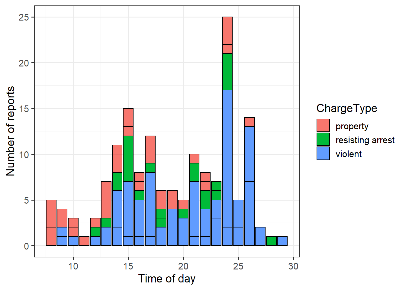
We see the consequences of adding 24 hours to some arrest times: Obviously there aren’t 30 hours in any day.
But we can use some ggplot tricks in scale_x_ to tweak (1) interval of hours displayed (breaks=) and (2) change the scale to a 2-hour increment that goes from 0800 to 2200, and then mindight, 0200, and 0400 (labels= and seq()).
Finally, we break the stacked bar graph into three panels for each charge type:
 hr_gg +
    scale_x_continuous(breaks=seq(8,28,2),
                       labels = c(seq(8,22,2),0,2,4 )) +
    scale_y_continuous(breaks=c(seq(1,20,3))) +
    facet_grid(GameDay ~ ChargeType,
               labeller = labeller(.rows = label_both)) +
    scale_fill_brewer(palette="Set1",
guide = FALSE) 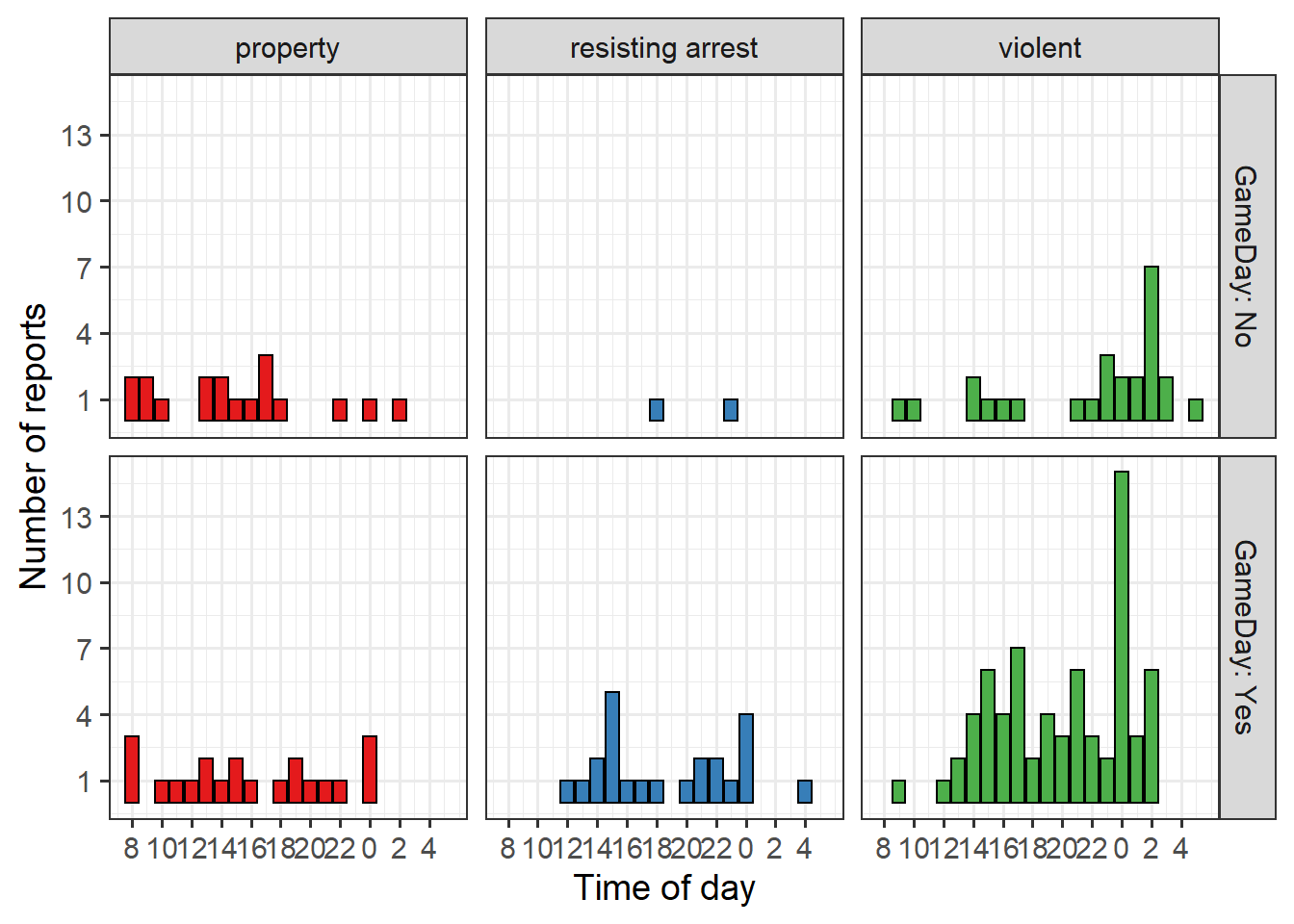
Note the use of labeller= to get very refined control of the labels for the facet rows.
Homework assignment
Work with a unique dataset on livestock behavior. Assignment posted to GitHub
An alternative would be to use
group_byandsummarizeto create a summary table and plot the bars with something likey = count, butstat = 'count'is a great option when creating such a table would be just for this one purpose.↩It would be easy for you to do this yourself at this point, using
mutate(other = case_when(...))↩as.Dateoperates only on calendar days and does not need time.↩If this happens with your data–an important variable of interest has
NA–you better look into it, not just filter it out!↩