Materials
Video lecture
Walking through the script
Remember, only run install.packages once per package, and do not include it in a .Rmd file.
install.packages("gridExtra")
install.packages("remotes")
pacman::p_load(tidyverse, vegan)
# Load, select, and scale data
data(varechem)
chem_s <-
select(varechem, N:Mo) %>%
scale(center=FALSE) # Fit cluster diagram on Euclidean distance matrix
chem_clust <-
chem_s %>%
vegdist("euc") %>%
hclust("ward.D2")GGplotting cluster analysis
  # Two add-on packages
    pacman::p_load(ggdendro, dendextend)
# ggplot2-style with ggdendro::ggdendrogram
ggdendrogram(chem_clust) + theme_minimal(16) +
labs(x = "Site",
y = "Euclidean distance") +
coord_flip() +
theme(panel.grid.major.y = element_blank(),
panel.grid.minor.y = element_blank())
  # requires dendextend
    chem_clust %>%
      as.dendrogram %>%
      set("branches_k_color", k = 5) %>%
      set("branches_lwd", 1.2) %>%
      as.ggdend( ) %>%
      ggplot(horiz=TRUE,
             offset_labels = -0.25 ) +
      theme_minimal(16) +
      labs(x = "Site",
           y = "Euclidean distance") +
      scale_y_continuous(position = "left") +
      theme(axis.text.y = element_blank(),
            panel.grid.major.y = element_blank(),
            panel.grid.minor.y = element_blank())
## Scale for 'y' is already present. Adding another scale for 'y', which will
## replace the existing scale.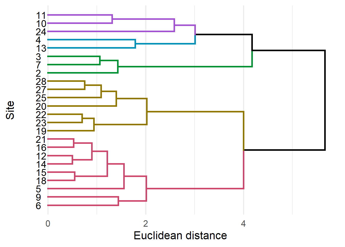
GGplotting ordinations
Getting set up
  # Load groups
  # (I just made some group assignments up, not from original data)
    man <- read_csv("https://github.com/devanmcg/IntroRangeR/raw/master/data/VareExample/Management.csv")
##
## -- Column specification --------------------------------------------------------
## cols(
## SampleID = col_character(),
## Pasture = col_double(),
## Treatment = col_double(),
## PastureName = col_character(),
## BurnSeason = col_character(),
## BareSoil = col_character()
## ) # Fit PCA
chem_pca <- capscale(chem_s ~ 1, "euc")
# Vector fitting
pca_hd <- envfit(chem_pca ~ Humdepth, varechem, choices = c(1:3)) # Extract scores
pca_spp <- # species only; sites come later
scores(chem_pca, display = "species") %>%
as.data.frame %>%
as_tibble(rownames="nutrient")
# Vector
pca_v <- scores(pca_hd, "vectors") %>%
as.data.frame %>%
round(3) %>%
as_tibble(rownames="gradient") # store scores in a list
pca_scores <- lst(species=pca_spp,
vectors=pca_v)
str(pca_scores)## List of 2
## $ species: tibble [11 x 3] (S3: tbl_df/tbl/data.frame)
## ..$ nutrient: chr [1:11] "N" "P" "K" "Ca" ...
## ..$ MDS1 : num [1:11] 0.0398 -0.1636 -0.1682 -0.3512 -0.268 ...
## ..$ MDS2 : num [1:11] 0.0803 -0.4519 -0.5351 -0.4537 -0.5217 ...
## $ vectors: tibble [1 x 4] (S3: tbl_df/tbl/data.frame)
## ..$ gradient: chr "Humdepth"
## ..$ MDS1 : num -0.553
## ..$ MDS2 : num -0.127
## ..$ MDS3 : num 0.104Load extension package for ordinations in ggplot
remotes::install_github("jfq3/ggordiplots" )
pacman::p_load(ggordiplots)
# If that doesn't work, just load the function itself:
  source("https://raw.githubusercontent.com/devanmcg/IntroRangeR/master/11_IntroMultivariate/ordinationsGGplot.R")
# View default plot (plot = TRUE)
gg_ordiplot(chem_pca, groups = man$BurnSeason,
spiders=TRUE, ellipse=FALSE, plot=TRUE)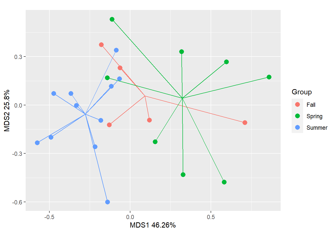
  # Store as an object (plot = FALSE)
    pca_gg <- gg_ordiplot(chem_pca, groups = man$BurnSeason,
                          plot=FALSE)
# Add spiderplot groups and species scores to list of scores
pca_scores$spiders <-
pca_gg$df_spiders %>%
rename(MDS1 = x, MDS2 = y) %>%
as_tibble
str(pca_scores)## List of 3
## $ species: tibble [11 x 3] (S3: tbl_df/tbl/data.frame)
## ..$ nutrient: chr [1:11] "N" "P" "K" "Ca" ...
## ..$ MDS1 : num [1:11] 0.0398 -0.1636 -0.1682 -0.3512 -0.268 ...
## ..$ MDS2 : num [1:11] 0.0803 -0.4519 -0.5351 -0.4537 -0.5217 ...
## $ vectors: tibble [1 x 4] (S3: tbl_df/tbl/data.frame)
## ..$ gradient: chr "Humdepth"
## ..$ MDS1 : num -0.553
## ..$ MDS2 : num -0.127
## ..$ MDS3 : num 0.104
## $ spiders: tibble [24 x 5] (S3: tbl_df/tbl/data.frame)
## ..$ Group : Factor w/ 3 levels "Fall","Spring",..: 1 1 1 1 1 2 2 2 2 2 ...
## ..$ cntr.x: num [1:24] 0.0918 0.0918 0.0918 0.0918 0.0918 ...
## ..$ cntr.y: num [1:24] 0.0565 0.0565 0.0565 0.0565 0.0565 ...
## ..$ MDS1 : num [1:24] 0.7106 0.1193 -0.0632 -0.1298 -0.1778 ...
## ..$ MDS2 : num [1:24] -0.1086 -0.0927 0.2308 -0.1217 0.3746 ...# Build up the ggplot
# The base plot.
# Note this is empty;
# we add data later (twice, actually)
ord_gg <- ggplot() + theme_bw(16) +
labs(x="MDS Axis 1",
y="MDS Axis 2") +
geom_vline(xintercept = 0, lty=3, color="darkgrey") +
geom_hline(yintercept = 0, lty=3, color="darkgrey") +
theme(panel.grid=element_blank(),
legend.position="none")
ord_gg + geom_point(data=pca_scores$spiders,
aes(x=MDS1, y=MDS2,
shape=Group,
colour=Group),
size=2)
  # Add environmental vector
    sites_gg <-
      ord_gg +
      geom_segment(data=pca_scores$vectors,
                   aes(x=0, y=0,
                       xend=MDS1,
                       yend=MDS2),
                   arrow=arrow(length = unit(0.03, "npc")),
                   lwd=1.5) +
      geom_text(data=pca_scores$vectors,
                aes(x=MDS1*0.9,
                    y=MDS2*0.9,
                    label=gradient),
                nudge_x = 0.06,
                nudge_y =-0.05,
                size=6, fontface="bold")
    sites_gg + geom_point(data=pca_scores$spiders,
                          aes(x=MDS1, y=MDS2,
                              shape=Group,
                              colour=Group),
                          size=2)
  # Add spiderplot grouping sites by burn season
    sites_gg <-
      sites_gg +
        geom_segment(data=pca_scores$spiders,
                     aes(x=cntr.x, y=cntr.y,
                         xend=MDS1, yend=MDS2,
                         color=Group),
                     size=1.2) +
        geom_point(data=pca_scores$spiders,
                   aes(x=MDS1, y=MDS2, bg=Group),
                   colour="black", pch=21,
                   size=3, stroke=2) +
        geom_label(data=pca_scores$spiders,
                   aes(x=cntr.x, y=cntr.y,
                       label=Group,
                       color=Group),
                   fontface="bold", size=4,
                   label.size = 0,
                   label.r = unit(0.5, "lines"))
    sites_gg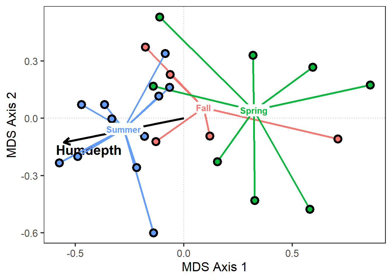
  # View species scores
    sites_gg + geom_label(data=pca_scores$species,
                          aes(x=MDS1,
                              y=MDS2,
                              label=nutrient),
                          label.padding=unit(0.1,"lines"),
                          label.size = 0,
                          fontface="bold", color="darkred")
  # Scale back species scores with x,y multiplier
    biplot_gg <-
      sites_gg +
      geom_label(data=pca_scores$species,
                 aes(x=MDS1*0.75,
                     y=MDS2*0.75,
                     label=nutrient),
                 label.padding=unit(0.1,"lines"),
                 label.size = 0,
                 fontface="bold", color="darkred")
    biplot_gg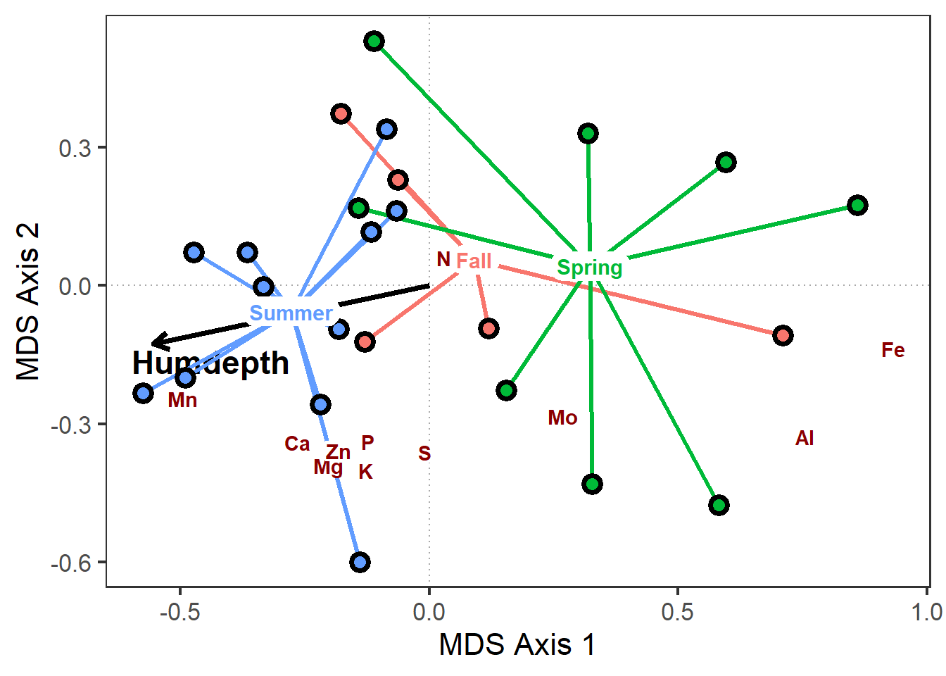
  # Adding species scores to a plot of groups & vectors
  # can get too cluttered; we're fortunate here the "species"
  # are two-character chemical symbols.
  # When they are so long or numerous as to clutter up the plot,
  # I often put them in a separate plot and only give their
  # locations in the site scores plot for reference:

  sites2_gg <-
    sites_gg +
      geom_point(data=pca_scores$species,
                 aes( x=MDS1*0.75,
                      y=MDS2*0.75),
                 shape="+", color="darkred", size=5)
  sites2_gg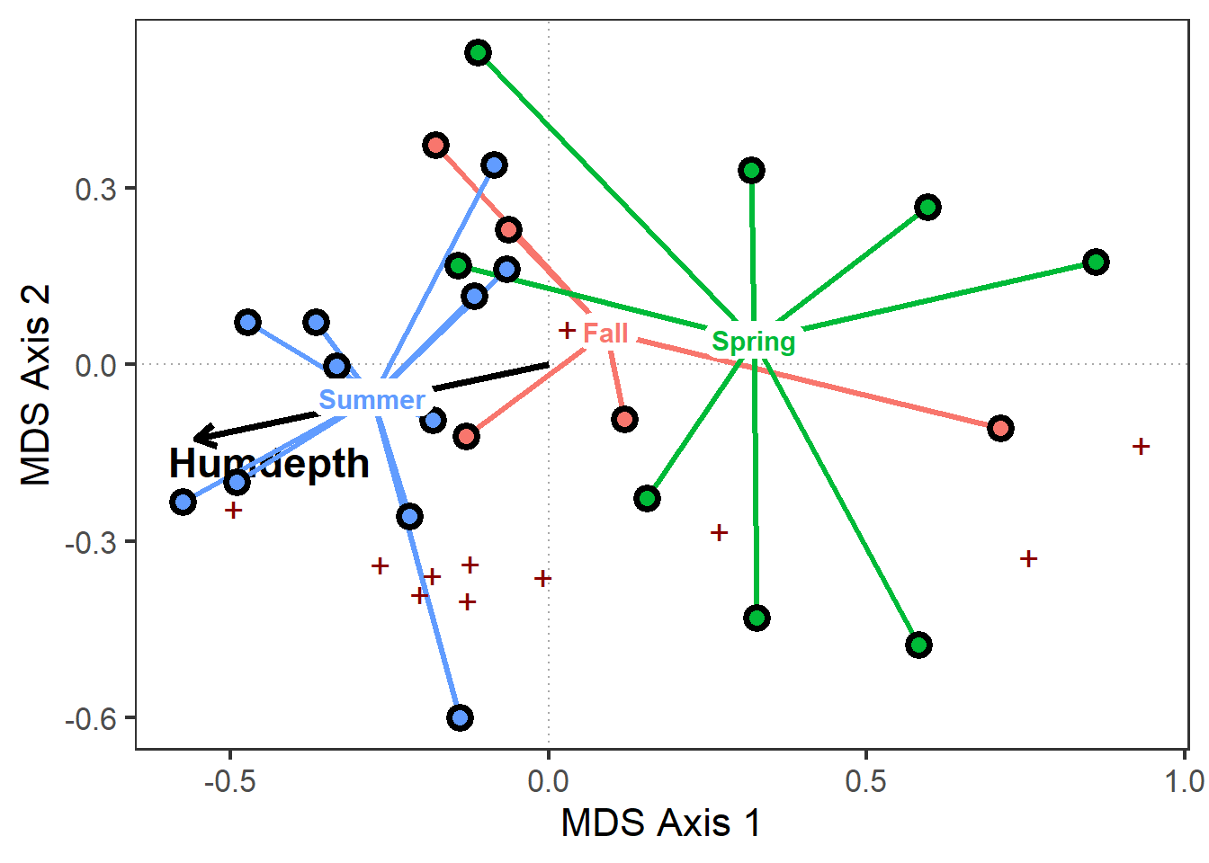
  # Make a separate graph of just species scores
  spp_gg <- ord_gg +
              geom_label(data=pca_scores$species,
                         aes(x=MDS1*0.75,
                             y=MDS2*0.75,
                             label=nutrient),
                         label.padding=unit(0.1,"lines"),
                         label.size = 0,
                         fontface="bold", color="darkred")
  spp_gg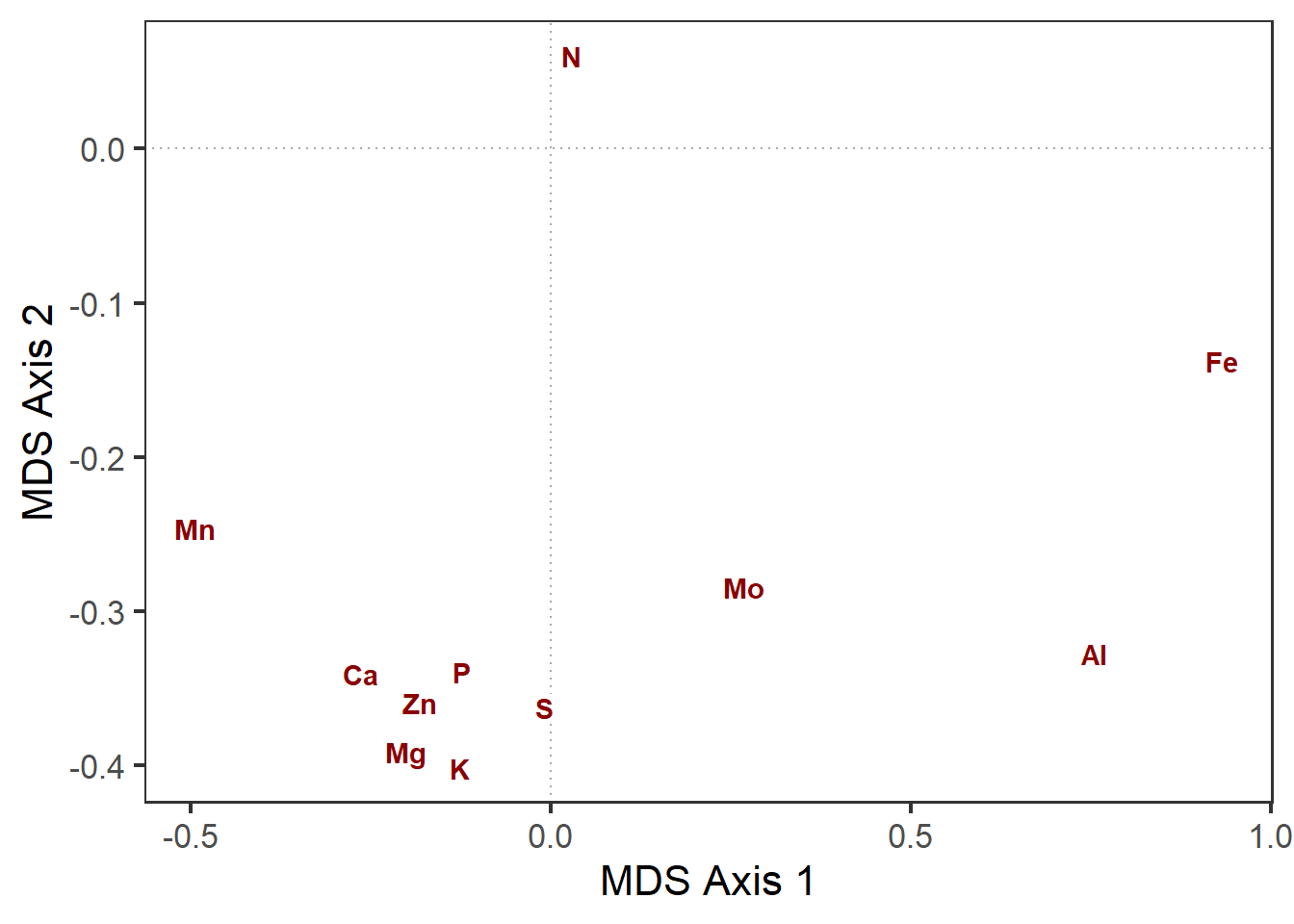
  # Then plot the species scores and (grouped) site scores
  # side-by-side with gridExtra::grid.arrange

  grid.arrange(spp_gg, sites2_gg, nrow=1)