Objectives
- Access data directly from Excel workbooks via readxl
- Combine familiar tidyverse verbs like
mutate()andfull_join()with new functions to manipulate data:- Combine (and split) identifying columns with
unite()andseparate() - Switch between long and wide data formats with
pivot_verbs - Split character strings into individual observations with
str_split()
- Combine (and split) identifying columns with
Walking through the script
pacman::p_load(tidyverse, readxl)
setwd("../R")
Remember: it is bad practice to use setwd() in a .Rmd file; rather, use full file paths.
Load data
Here are some new tricks to load data directly from an Excel workbook (.xlsx) without exporting and saving individual worksheets as .csv files.
For convenience, define the file path as an object:
xl_file = "./data/VareExample.xlsx" Use full path (no .) in an .Rmd file.
Begin by importing tibbles from specific worksheets in the .xlsx file into tibble using read_excel() in readxl:
spp_tbl <- read_excel(xl_file, "SpeciesData")
man_tbl <- read_excel(xl_file, "Management")
Remember a tibble object doesn’t need str() or head():
spp_tbl ## # A tibble: 24 x 47
## Pasture Treatment Point Callvulg Empenigr Rhodtome Vaccmyrt Vaccviti Pinusylv
## <dbl> <dbl> <dbl> <dbl> <dbl> <dbl> <dbl> <dbl> <dbl>
## 1 1 1 1 0.55 11.1 0 0 17.8 0.07
## 2 2 2 1 0.67 0.17 0 0.35 12.1 0.12
## 3 2 2 2 0.1 1.55 0 0 13.5 0.25
## 4 2 2 3 0 15.1 2.42 5.92 16.0 0
## 5 2 2 4 0 12.7 0 0 23.7 0.03
## 6 2 2 5 0 8.92 0 2.42 10.3 0.12
## 7 2 2 6 4.73 5.12 1.55 6.05 12.4 0.1
## 8 2 2 7 4.47 7.33 0 2.15 4.33 0.1
## 9 2 2 8 0 1.63 0.35 18.3 7.13 0.05
## 10 1 1 2 24.1 1.9 0.07 0.22 5.3 0.12
## # … with 14 more rows, and 38 more variables: Descflex <dbl>, Betupube <dbl>,
## # Vacculig <dbl>, Diphcomp <dbl>, Dicrsp <dbl>, Dicrfusc <dbl>,
## # Dicrpoly <dbl>, Hylosple <dbl>, Pleuschr <dbl>, Polypili <dbl>,
## # Polyjuni <dbl>, Polycomm <dbl>, Pohlnuta <dbl>, Ptilcili <dbl>,
## # Barbhatc <dbl>, Cladarbu <dbl>, Cladrang <dbl>, Cladstel <dbl>,
## # Cladunci <dbl>, Cladcocc <dbl>, Cladcorn <dbl>, Cladgrac <dbl>,
## # Cladfimb <dbl>, Cladcris <dbl>, Cladchlo <dbl>, Cladbotr <dbl>,
## # Cladamau <dbl>, Cladsp <dbl>, Cetreric <dbl>, Cetrisla <dbl>,
## # Flavniva <dbl>, Nepharct <dbl>, Stersp <dbl>, Peltapht <dbl>,
## # Icmaeric <dbl>, Cladcerv <dbl>, Claddefo <dbl>, Cladphyl <dbl>man_tbl ## # A tibble: 24 x 6
## SampleID Pasture Treatment PastureName BurnSeason BareSoil
## <chr> <dbl> <dbl> <chr> <chr> <chr>
## 1 1.1.1 1 1 North Spring 42.5, 43.1, 43.9
## 2 2.2.1 2 2 South Summer 22.4, 23.9, 23.6
## 3 2.2.2 2 2 South Summer 20.2, 22.4, 21.2
## 4 2.2.3 2 2 South Summer 18.0, 18.7
## 5 2.2.4 2 2 South Summer 45.6, 47.2, 46
## 6 2.2.5 2 2 South Summer 39.4, 36.1, 40.5
## 7 2.2.6 2 2 South Summer 22.3, 24.1, 23.0
## 8 2.2.7 2 2 South Summer 29.1, 29.8
## 9 2.2.8 2 2 South Summer 17.4, 18.2, 17.6
## 10 1.1.2 1 1 North Spring 28.1, 30.4, 29.9
## # … with 14 more rowsModifying data with tidyverse
Remember that a primary objective of this course is to help you do your data manipulation “on the fly” and eliminate the need to go back to your raw data and make the manipulations in Excel. Such clicky-clicky operations are difficult to trace and repeat. tidyverse allows us to create reproducible and transparent workflows.
Creating columns
As an example of how we can create variables by combining columns that already exist, we take up the common issue of needing a unique ID for every single row of data. This is often the case when your samples come from some complex nested experimental structure, but the lab needs a single identifier to run samples and return the results to you.
Here we create a unique sample ID column in spp_d from three existing columns with the unite() verb:
spp_tbl <- unite(data=spp_tbl,
                 col="SampleID",
               c("Pasture", "Treatment", "Point"),
               sep=".")
spp_tbl
## # A tibble: 24 x 45
## SampleID Callvulg Empenigr Rhodtome Vaccmyrt Vaccviti Pinusylv Descflex
## <chr> <dbl> <dbl> <dbl> <dbl> <dbl> <dbl> <dbl>
## 1 1.1.1 0.55 11.1 0 0 17.8 0.07 0
## 2 2.2.1 0.67 0.17 0 0.35 12.1 0.12 0
## 3 2.2.2 0.1 1.55 0 0 13.5 0.25 0
## 4 2.2.3 0 15.1 2.42 5.92 16.0 0 3.7
## 5 2.2.4 0 12.7 0 0 23.7 0.03 0
## 6 2.2.5 0 8.92 0 2.42 10.3 0.12 0.02
## 7 2.2.6 4.73 5.12 1.55 6.05 12.4 0.1 0.78
## 8 2.2.7 4.47 7.33 0 2.15 4.33 0.1 0
## 9 2.2.8 0 1.63 0.35 18.3 7.13 0.05 0.4
## 10 1.1.2 24.1 1.9 0.07 0.22 5.3 0.12 0
## # … with 14 more rows, and 37 more variables: Betupube <dbl>, Vacculig <dbl>,
## # Diphcomp <dbl>, Dicrsp <dbl>, Dicrfusc <dbl>, Dicrpoly <dbl>,
## # Hylosple <dbl>, Pleuschr <dbl>, Polypili <dbl>, Polyjuni <dbl>,
## # Polycomm <dbl>, Pohlnuta <dbl>, Ptilcili <dbl>, Barbhatc <dbl>,
## # Cladarbu <dbl>, Cladrang <dbl>, Cladstel <dbl>, Cladunci <dbl>,
## # Cladcocc <dbl>, Cladcorn <dbl>, Cladgrac <dbl>, Cladfimb <dbl>,
## # Cladcris <dbl>, Cladchlo <dbl>, Cladbotr <dbl>, Cladamau <dbl>,
## # Cladsp <dbl>, Cetreric <dbl>, Cetrisla <dbl>, Flavniva <dbl>,
## # Nepharct <dbl>, Stersp <dbl>, Peltapht <dbl>, Icmaeric <dbl>,
## # Cladcerv <dbl>, Claddefo <dbl>, Cladphyl <dbl>The opposite of unite() is separate():
separate(spp_tbl,
         SampleID,
         c("Pasture","Treatment","Point"))
## # A tibble: 24 x 47
## Pasture Treatment Point Callvulg Empenigr Rhodtome Vaccmyrt Vaccviti Pinusylv
## <chr> <chr> <chr> <dbl> <dbl> <dbl> <dbl> <dbl> <dbl>
## 1 1 1 1 0.55 11.1 0 0 17.8 0.07
## 2 2 2 1 0.67 0.17 0 0.35 12.1 0.12
## 3 2 2 2 0.1 1.55 0 0 13.5 0.25
## 4 2 2 3 0 15.1 2.42 5.92 16.0 0
## 5 2 2 4 0 12.7 0 0 23.7 0.03
## 6 2 2 5 0 8.92 0 2.42 10.3 0.12
## 7 2 2 6 4.73 5.12 1.55 6.05 12.4 0.1
## 8 2 2 7 4.47 7.33 0 2.15 4.33 0.1
## 9 2 2 8 0 1.63 0.35 18.3 7.13 0.05
## 10 1 1 2 24.1 1.9 0.07 0.22 5.3 0.12
## # … with 14 more rows, and 38 more variables: Descflex <dbl>, Betupube <dbl>,
## # Vacculig <dbl>, Diphcomp <dbl>, Dicrsp <dbl>, Dicrfusc <dbl>,
## # Dicrpoly <dbl>, Hylosple <dbl>, Pleuschr <dbl>, Polypili <dbl>,
## # Polyjuni <dbl>, Polycomm <dbl>, Pohlnuta <dbl>, Ptilcili <dbl>,
## # Barbhatc <dbl>, Cladarbu <dbl>, Cladrang <dbl>, Cladstel <dbl>,
## # Cladunci <dbl>, Cladcocc <dbl>, Cladcorn <dbl>, Cladgrac <dbl>,
## # Cladfimb <dbl>, Cladcris <dbl>, Cladchlo <dbl>, Cladbotr <dbl>,
## # Cladamau <dbl>, Cladsp <dbl>, Cetreric <dbl>, Cetrisla <dbl>,
## # Flavniva <dbl>, Nepharct <dbl>, Stersp <dbl>, Peltapht <dbl>,
## # Icmaeric <dbl>, Cladcerv <dbl>, Claddefo <dbl>, Cladphyl <dbl>Wide vs long formats
Data frames are generally arranged in one of two formats: Wide or long.
Long data are stored in a column of values, which are identified by various groups with any number of categorical columns.
This format is common for univariate statistical analyses, and is conducive to using ggplot by mapping aesthetics like shape, color, or facet to the columns.
Wide data have a column for each type of data, which are often identified by the variable name as the column header. This is a necessary format for multivariate analyses and is the way many community or trait data are stored.
Indeed, spp_tbl is in wide format, with one column for each species:
| SampleID | Callvulg | Empenigr | Rhodtome | Vaccmyrt | Vaccviti | Pinusylv |
|---|---|---|---|---|---|---|
| 1.1.1 | 0.55 | 11.13 | 0 | 0 | 17.8 | 0.07 |
| 2.2.1 | 0.67 | 0.17 | 0 | 0.35 | 12.13 | 0.12 |
| 2.2.2 | 0.1 | 1.55 | 0 | 0 | 13.47 | 0.25 |
| 2.2.3 | 0 | 15.13 | 2.42 | 5.92 | 15.97 | 0 |
| 2.2.4 | 0 | 12.68 | 0 | 0 | 23.73 | 0.03 |
pivot_longer() brings wide data into long format.1
It works by identifying the two new columns to create (species and abundance) and any columns to exclude from the stacking operation are preceded by -; at least one allows unique row identifiers (in this case, our new SampleID column):
spp_long <- pivot_longer(spp_tbl,
                         names_to = "species",
                         values_to = "abundance",
                         -SampleID)
spp_long
## # A tibble: 1,056 x 3
## SampleID species abundance
## <chr> <chr> <dbl>
## 1 1.1.1 Callvulg 0.55
## 2 1.1.1 Empenigr 11.1
## 3 1.1.1 Rhodtome 0
## 4 1.1.1 Vaccmyrt 0
## 5 1.1.1 Vaccviti 17.8
## 6 1.1.1 Pinusylv 0.07
## 7 1.1.1 Descflex 0
## 8 1.1.1 Betupube 0
## 9 1.1.1 Vacculig 1.6
## 10 1.1.1 Diphcomp 2.07
## # … with 1,046 more rowsAnd just to demonstrate how we can undo the operation using pivot_wider():
pivot_wider(spp_long,
            names_from = "species",
            values_from = "abundance")
## # A tibble: 24 x 45
## SampleID Callvulg Empenigr Rhodtome Vaccmyrt Vaccviti Pinusylv Descflex
## <chr> <dbl> <dbl> <dbl> <dbl> <dbl> <dbl> <dbl>
## 1 1.1.1 0.55 11.1 0 0 17.8 0.07 0
## 2 2.2.1 0.67 0.17 0 0.35 12.1 0.12 0
## 3 2.2.2 0.1 1.55 0 0 13.5 0.25 0
## 4 2.2.3 0 15.1 2.42 5.92 16.0 0 3.7
## 5 2.2.4 0 12.7 0 0 23.7 0.03 0
## 6 2.2.5 0 8.92 0 2.42 10.3 0.12 0.02
## 7 2.2.6 4.73 5.12 1.55 6.05 12.4 0.1 0.78
## 8 2.2.7 4.47 7.33 0 2.15 4.33 0.1 0
## 9 2.2.8 0 1.63 0.35 18.3 7.13 0.05 0.4
## 10 1.1.2 24.1 1.9 0.07 0.22 5.3 0.12 0
## # … with 14 more rows, and 37 more variables: Betupube <dbl>, Vacculig <dbl>,
## # Diphcomp <dbl>, Dicrsp <dbl>, Dicrfusc <dbl>, Dicrpoly <dbl>,
## # Hylosple <dbl>, Pleuschr <dbl>, Polypili <dbl>, Polyjuni <dbl>,
## # Polycomm <dbl>, Pohlnuta <dbl>, Ptilcili <dbl>, Barbhatc <dbl>,
## # Cladarbu <dbl>, Cladrang <dbl>, Cladstel <dbl>, Cladunci <dbl>,
## # Cladcocc <dbl>, Cladcorn <dbl>, Cladgrac <dbl>, Cladfimb <dbl>,
## # Cladcris <dbl>, Cladchlo <dbl>, Cladbotr <dbl>, Cladamau <dbl>,
## # Cladsp <dbl>, Cetreric <dbl>, Cetrisla <dbl>, Flavniva <dbl>,
## # Nepharct <dbl>, Stersp <dbl>, Peltapht <dbl>, Icmaeric <dbl>,
## # Cladcerv <dbl>, Claddefo <dbl>, Cladphyl <dbl>These are extremely useful functions that go a long way towards reducing the number of versions of your data you need to store (and keep track of, and recreate…) outside of \({\bf\textsf{R}}\) in programs like Excel.
Manipulating string variables
Our species data only include abundance of each species. To look for patterns in these data, we need to have more information about each sample.
man_tbl has data on environmental variables related to management practices:
man_tbl## # A tibble: 24 x 6
## SampleID Pasture Treatment PastureName BurnSeason BareSoil
## <chr> <dbl> <dbl> <chr> <chr> <chr>
## 1 1.1.1 1 1 North Spring 42.5, 43.1, 43.9
## 2 2.2.1 2 2 South Summer 22.4, 23.9, 23.6
## 3 2.2.2 2 2 South Summer 20.2, 22.4, 21.2
## 4 2.2.3 2 2 South Summer 18.0, 18.7
## 5 2.2.4 2 2 South Summer 45.6, 47.2, 46
## 6 2.2.5 2 2 South Summer 39.4, 36.1, 40.5
## 7 2.2.6 2 2 South Summer 22.3, 24.1, 23.0
## 8 2.2.7 2 2 South Summer 29.1, 29.8
## 9 2.2.8 2 2 South Summer 17.4, 18.2, 17.6
## 10 1.1.2 1 1 North Spring 28.1, 30.4, 29.9
## # … with 14 more rowsThe categorical variables are self-explanatory, but BareSoil is confusing.
These are numeric data, but are stored as a chr character vector.
Each entry in the BareSoil vector is actually a character string comprised of three observations, separated by commas.
To use these data, we need to split the observations into their own numeric vectors.
There are several functions for working with character strings in both tidyverse and base \({\bf\textsf{R}}\).2.
Together, the str_ functions are powerful tools for accomplishing all sorts of tasks with text data.
We scratch the surface of text manipulation with str_split(), which breaks text strings apart on a specified character.
But the output of str_split() is a list of items broken up from the original character string, so we immediately follow up with another tidyverse verb, unnest(), to put each observation on its own line:
man_tbl <-
  man_tbl %>%
    mutate(BareSoil = str_split(BareSoil, ",")) %>%
      unnest(BareSoil)
man_tbl
## # A tibble: 70 x 6
## SampleID Pasture Treatment PastureName BurnSeason BareSoil
## <chr> <dbl> <dbl> <chr> <chr> <chr>
## 1 1.1.1 1 1 North Spring "42.5"
## 2 1.1.1 1 1 North Spring " 43.1"
## 3 1.1.1 1 1 North Spring " 43.9"
## 4 2.2.1 2 2 South Summer "22.4"
## 5 2.2.1 2 2 South Summer " 23.9"
## 6 2.2.1 2 2 South Summer " 23.6"
## 7 2.2.2 2 2 South Summer "20.2"
## 8 2.2.2 2 2 South Summer " 22.4"
## 9 2.2.2 2 2 South Summer " 21.2"
## 10 2.2.3 2 2 South Summer "18.0"
## # … with 60 more rowsConveniently, unnest() also automatically copies entries from the other columns; note how SampleID is repeated.
Now we have our single observations, but they are still stored as characters and must be converted to numeric:
man_tbl <- mutate(man_tbl, BareSoil = as.numeric(BareSoil))
man_tbl
## # A tibble: 70 x 6
## SampleID Pasture Treatment PastureName BurnSeason BareSoil
## <chr> <dbl> <dbl> <chr> <chr> <dbl>
## 1 1.1.1 1 1 North Spring 42.5
## 2 1.1.1 1 1 North Spring 43.1
## 3 1.1.1 1 1 North Spring 43.9
## 4 2.2.1 2 2 South Summer 22.4
## 5 2.2.1 2 2 South Summer 23.9
## 6 2.2.1 2 2 South Summer 23.6
## 7 2.2.2 2 2 South Summer 20.2
## 8 2.2.2 2 2 South Summer 22.4
## 9 2.2.2 2 2 South Summer 21.2
## 10 2.2.3 2 2 South Summer 18
## # … with 60 more rowsAs your skills develop, you’ll anticipate this behavior of character-manipulation functions and intuitively add the mutate( ... as.numeric) step in your pipe operation, just as one adds unnest() after str_split().
A final step remains before we can add this information to our data on species abundance. At each sample point, we have three observations of bare soil exposure, but only one observation of abundance for each species. We must summarize the bare soil data to fit the length of each sample number in the dataset with the fewest observations per sample (in this case, 1):
man_tbl <-
  man_tbl %>%
    group_by(SampleID, PastureName, BurnSeason) %>%
      summarise(BareSoil = mean(BareSoil)) %>%
        ungroup
man_tbl
## # A tibble: 24 x 4
## SampleID PastureName BurnSeason BareSoil
## <chr> <chr> <chr> <dbl>
## 1 1.1.1 North Spring 43.2
## 2 1.1.2 North Spring 29.5
## 3 1.1.3 North Spring 18.7
## 4 1.1.4 North Spring 8.47
## 5 1.1.5 North Spring 5.43
## 6 1.1.6 North Spring 3.63
## 7 1.1.7 North Spring 21.4
## 8 1.1.8 North Spring 6.40
## 9 1.3.1 North Fall 0.0367
## 10 1.3.2 North Fall 5.66
## # … with 14 more rowsWe summarized with mean() above, but the “best” function will depend on your research question or protocol. Alternatives include median(), min(), max(), etc.
Take a minute to think of how this string-splitting operation could change your entire data workflow.
Consider the typical datasheet, with blanks for each desired observation, and an Access-type data form, with a corresponding number of blanks.
What if some of those observations were not recorded?
Now recall from the first lesson how we used length() to allow \({\bf\textsf{R}}\) to determine how many observations should be used to divide the sum by, rather than hard-coding 5.
Knowing how one will manipulate their data once they are in the computer can open up new possibilities for flexible data recording and entry.
For example, instead of a confusing datasheet with many blanks, consider writing a number of observations on a single line of the datasheet, which can be entered as a character string with observations separated by punctuation like a comma.
With unnest() and summarize(), it doesn’t matter how many observations are actually recorded; like length(), this workflow is flexible and allows for more intuitively-organized datasheets.
Consolidate into one object
Now, we join the two data sets on the SampleID column:
full_join(man_tbl,
          spp_tbl,
          by="SampleID")
## # A tibble: 24 x 48
## SampleID PastureName BurnSeason BareSoil Callvulg Empenigr Rhodtome Vaccmyrt
## <chr> <chr> <chr> <dbl> <dbl> <dbl> <dbl> <dbl>
## 1 1.1.1 North Spring 43.2 0.55 11.1 0 0
## 2 1.1.2 North Spring 29.5 24.1 1.9 0.07 0.22
## 3 1.1.3 North Spring 18.7 0 5.3 0 0
## 4 1.1.4 North Spring 8.47 0 0.13 0 0
## 5 1.1.5 North Spring 5.43 0.3 5.75 0 0
## 6 1.1.6 North Spring 3.63 0.03 3.65 0 0
## 7 1.1.7 North Spring 21.4 3.4 0.63 0 0
## 8 1.1.8 North Spring 6.40 2.37 0.67 0 0
## 9 1.3.1 North Fall 0.0367 0.05 9.3 0 0
## 10 1.3.2 North Fall 5.66 0 3.47 0 0.25
## # … with 14 more rows, and 40 more variables: Vaccviti <dbl>, Pinusylv <dbl>,
## # Descflex <dbl>, Betupube <dbl>, Vacculig <dbl>, Diphcomp <dbl>,
## # Dicrsp <dbl>, Dicrfusc <dbl>, Dicrpoly <dbl>, Hylosple <dbl>,
## # Pleuschr <dbl>, Polypili <dbl>, Polyjuni <dbl>, Polycomm <dbl>,
## # Pohlnuta <dbl>, Ptilcili <dbl>, Barbhatc <dbl>, Cladarbu <dbl>,
## # Cladrang <dbl>, Cladstel <dbl>, Cladunci <dbl>, Cladcocc <dbl>,
## # Cladcorn <dbl>, Cladgrac <dbl>, Cladfimb <dbl>, Cladcris <dbl>,
## # Cladchlo <dbl>, Cladbotr <dbl>, Cladamau <dbl>, Cladsp <dbl>,
## # Cetreric <dbl>, Cetrisla <dbl>, Flavniva <dbl>, Nepharct <dbl>,
## # Stersp <dbl>, Peltapht <dbl>, Icmaeric <dbl>, Cladcerv <dbl>,
## # Claddefo <dbl>, Cladphyl <dbl>Now that the data are in the same format, fit to the same number of observations per sample point, and combined, we can easily plot a variable from one sheet in the original Excel file by data from another sheet:
full_join(man_tbl,
          spp_tbl,
          "SampleID") %>%
mutate(GroundCover = 100 - BareSoil) %>%
  filter(BurnSeason != "Fall") %>%
  ggplot(aes(x = GroundCover,
             y = Empenigr)) +
    theme_bw(16) +
      geom_smooth(method = "lm", se = F) +
      geom_point(size=3) +
    facet_wrap(~BurnSeason,
               scales = "free_x") +
    labs(x = "Soil coverage (%)",
         y = "Empetrum nigrum",
        title = "E. nigrum abundance by ground cover & burn season")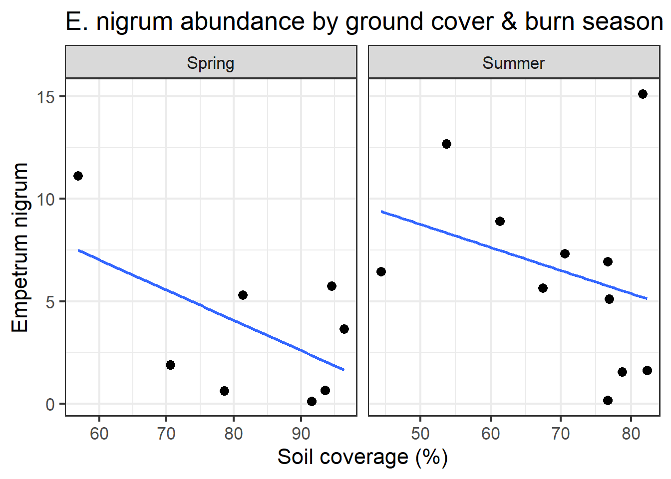
Pay close attention to that chunk. It includes several shortcuts facilitated by tidyverse:
- Note how the
joincan pour right into a pipe and down into a call toggplot(). - Notice also how we use
mutate()to make the bare soil more intuitive. For example, we might be more interested in how ground cover affects a species and simply use bare ground exposure as a proxy for ground cover, in which case we’d be more interested in plotting the inverse of the data at hand.