Walking through the script
Working directories
Working directories help pull data from, and save to, specific files. One can always see what your current working directory is:
getwd() One can also see what is currently in \({\bf\textsf{R}}\)’s global environment:
ls() Use setwd() to change the working directory.
For this course, I recommend having a folder called R in a thumbdrive or on your desktop.
setwd("E:/R/") Note that one must use a single forward slash / or double back slash \\ instead of the single back slash \ that is the default for file paths in Windows.
Saving objects
The save() function saves specific objects.
This can be a good idea after after importing large datasets, performing extensive data manipulations, or after running an operation that took a long time to chug.
One can define file= as a full file string, or use ./ as a shortcut to the working directory.
This is especially convenient if the file is to be saved to a folder that is nested under many others.
save(file_name, file="./file_name.Rdata") To load an object previously saved to the working directory into the current environment, use load():
load("./file_name.Rdata") One can also save everything that is currently in the workspace, aka global environment (everything returned by ls()):
save.image()Depending on your R studio settings, you will likely be asked if you’d like to do this when you close an R studio session.
At first this makes sense–it has been drilled into us to save, save, save!
But there is a strong argument not to save an R workspace, or even objects.
Basically, the point of reproducible code is to be able to repeat operations, and it is risky to load up a previous work session without knowing exactly what prior manipulations have been performed (e.g., are the columns in the DataSummarized.Rdata file you made last year means or medians? Standard deviation or standard error??)
Packages
\({\bf\textsf{R}}\) functions are grouped into libraries, also known as packages.
Even functions that come with \({\bf\textsf{R}}\) by default are assigned to packages: sum is in package base; lm (for linear model fitting) is in the pre-loaded package stats; fitdistr (for finding moments of data distributions) is in the pre-packaged but not automatically-loaded package MASS.
Packages are also the main means by which the global \({\bf\textsf{R}}\) community shares new functions that build on the open-source capacity of base \({\bf\textsf{R}}\). Other users can build packages around the custom functions they developed and share on platforms like the Comprehensive R Archive Network (CRAN) or GitHub.
Using external packages requires them to be downloaded to one’s local machine.
Base \({\bf\textsf{R}}\) provides the function install.packages() to fetch packages from CRAN and make them available to \({\bf\textsf{R}}\) on one’s computer.
I often prefer–and especially for this class–to use a package to manage my packages. So let’s install it real quick once using the base method:
install.packages("pacman")Outside of R studio, one might be prompted to select a source from which to download a copy of the package among all of the global repositories. One can select anywhere, but might consider the one that is geographically closest.
Once a package is installed, we will generally refer to it as a library, if only because that is the function that invokes an installed package for use in a specific \({\bf\textsf{R}}\) session.
library(pacman) Now, all of the functions included in pacman are available for use in the current \({\bf\textsf{R}}\) session.
Each time \({\bf\textsf{R}}\) is restarted, libraries based on external packages must be called, but the package only needs to be downloaded once.
I strongly recommend not re-installing a package every time you start up \({\bf\textsf{R}}\) for class, so avoid ever including a call to install.packages() in your script, especially for homework.
You must also load packages in an R markdown file if a function from the package is used in a code chunk, even if you have the package loaded in your current \({\bf\textsf{R}}\) session.
Uncertainty about whether I or you all have a given package installed at a given time is what prompts my allegiance to pacman.
The p_load() function first checks to see if the package is available locally. If it is, p_load() calls library() for you.
If the package is not available locally, p_load() runs install.packages() for you then runs library() automatically.
Here we use p_load() to get us ready to use functions in the dplyr package:
p_load(dplyr)Sometimes one wants only to use a specific function from an external package once, and does not want to load the entire library into the current workspace.
This is frequently the case when two packages have functions with the same name, but perform different operations.
Such conflicts are very annoying, and can seriously muck up a carefully-crafted script.
Two frequent conflicts are between select in MASS and dplyr, or rename in plyr and dplyr.
To avoid conflict, one can use a function from a package without loading the library by using the package::function convention:
pacman::p_load(dplyr) Here we get all of the functionality of p_load() without bringing anything from pacman into the current environment.
Diagnostic data functions
We’ll learn how to load data into \({\bf\textsf{R}}\) shortly. For now we are going to play with one of several data sets that comes with \({\bf\textsf{R}}\) by default, for examples such as this one.
We’ll begin by using a few functions to check out the cars dataset.
Things we might be interested in knowing about the data include:
- How many columns of data are included? How many rows?
- What type of object is it? \({\bf\textsf{R}}\) has several data types that support different types of operations.
- What types of data are included–are they numbers? Words? Codes?
dim() gives us the dimensions of the data–the number of rows, and the number of columns:
dim(cars)## [1] 50 2\({\bf\textsf{R}}\) allows one to assign a name to each column of a data frame like cars, and the names() function shows us what they are:
names(cars)## [1] "speed" "dist"To get a peek at both the names and the first six lines of the data, just to see what sort of stuff is in there, we have head() (and tail() to look at the bottom):
head(cars) ## speed dist
## 1 4 2
## 2 4 10
## 3 7 4
## 4 7 22
## 5 8 16
## 6 9 10tail(cars) ## speed dist
## 45 23 54
## 46 24 70
## 47 24 92
## 48 24 93
## 49 24 120
## 50 25 85Note the (unnamed) column of row numbers along the left, and how the output of tail() corresponds with the output of dim().
Classes
Data in \({\bf\textsf{R}}\) are stored as various classes.
Several are described in the video, and in various places online.
We will mostly use data.frames and the tidyverse equivalent tibble.
Determine which class an object is stored as with class():
class(cars)## [1] "data.frame"Data within objects are also assigned to classes, and the class() function also identifies how vectors are stored, as well.
The $ character is a reserved operator in \({\bf\textsf{R}}\) that specifies a combination of a column in an object:
class(cars$speed)## [1] "numeric"str() is a comprehensive function that combines the output of most of the functions above:
str(cars) ## 'data.frame': 50 obs. of 2 variables:
## $ speed: num 4 4 7 7 8 9 10 10 10 11 ...
## $ dist : num 2 10 4 22 16 10 18 26 34 17 ...From this output we see that
carsis adata.frame…- 50 rows long and 2 columns wide,
- with two
numeric columns … - …that are called
speedanddist - And we can see the first 10 values of each vector
The summary() function is really important in viewing the results of statistical analyses that are stored as objects.
When called on data objects, it returns summary statistics for the vectors therein:
summary(cars)Working with specific columns
Whereas head(object) returns the top six rows of all vectors in the data frame, the $ operator can be included to return just the top six items in a specific named vector:
head(cars) ## speed dist
## 1 4 2
## 2 4 10
## 3 7 4
## 4 7 22
## 5 8 16
## 6 9 10head(cars$speed) ## [1] 4 4 7 7 8 9To specify a vector by position instead of by column name, \({\bf\textsf{R}}\) provides a convention that uses the square brackets [ ] and does not use the $ or column names:
head(cars[1]) ## speed
## 1 4
## 2 4
## 3 7
## 4 7
## 5 8
## 6 9While we don’t often need to refer to a column by position, the square bracket convention is extremely useful when the name of the column is dynamic, or needs to change, and we don’t want it hard-coded.
We can define a variable that represents the column name, and feed it to the head() function via double square brackets [[ ]]:
column = "speed"
head(cars[[column]])
## [1] 4 4 7 7 8 9Consider an example in which we have a program written to apply an operation to each column in a data frame, and we want it to be flexible enough to accommodate data frames with a different number of columns, or columns that occur in any order.
We can define a vector of the names of the data frame columns:
columns <- names(cars)
columns
## [1] "speed" "dist"length(columns)## [1] 2Then use a for loop to work through each column in the data frame:
    for( i in 1:length(columns)) {
      column = columns[i]
      print(head(cars[[column]]))
    }
## [1] 4 4 7 7 8 9
## [1] 2 10 4 22 16 10This is a silly, trivial little script but it demonstrates the principle of dynamic column names.
Evaluating specific rows and cells
We’ve talked about how \({\bf\textsf{R}}\) is built to work around vectors, which are columns in most data classes.
Thus it shouldn’t be surprising that the numbers in square brackets are assumed to refer to columns.
One can refer to a row, but the numeral must be followed by a comma ,.
The square bracket convention is actually [X,Y] coordinates, as in mapping out a spreadsheet as if it were a grid, but again, with the focus on columns, \({\bf\textsf{R}}\) doesn’t make us use [,Y].
cars[1,] ## speed dist
## 1 4 2The single colon : allows one to define a range:
cars[1:3,] ## speed dist
## 1 4 2
## 2 4 10
## 3 7 4cars[3:5,] ## speed dist
## 3 7 4
## 4 7 22
## 5 8 16Individual cells can be referred to by using the full [X,Y] notation:
cars[5,2] ## [1] 16A more complex dataset
cars has two numeric columns.
mtcars, though–a dataset derived from Motor Trend magazine’s test of several 1974 model year automobiles–has several more columns:
str(mtcars)## 'data.frame': 32 obs. of 11 variables:
## $ mpg : num 21 21 22.8 21.4 18.7 18.1 14.3 24.4 22.8 19.2 ...
## $ cyl : num 6 6 4 6 8 6 8 4 4 6 ...
## $ disp: num 160 160 108 258 360 ...
## $ hp : num 110 110 93 110 175 105 245 62 95 123 ...
## $ drat: num 3.9 3.9 3.85 3.08 3.15 2.76 3.21 3.69 3.92 3.92 ...
## $ wt : num 2.62 2.88 2.32 3.21 3.44 ...
## $ qsec: num 16.5 17 18.6 19.4 17 ...
## $ vs : num 0 0 1 1 0 1 0 1 1 1 ...
## $ am : num 1 1 1 0 0 0 0 0 0 0 ...
## $ gear: num 4 4 4 3 3 3 3 4 4 4 ...
## $ carb: num 4 4 1 1 2 1 4 2 2 4 ...All columns are stored as numeric, as well, and are indeed numbers.
We can perform a similar query as above, using summary():
summary(mtcars)## mpg cyl disp hp
## Min. :10.40 Min. :4.000 Min. : 71.1 Min. : 52.0
## 1st Qu.:15.43 1st Qu.:4.000 1st Qu.:120.8 1st Qu.: 96.5
## Median :19.20 Median :6.000 Median :196.3 Median :123.0
## Mean :20.09 Mean :6.188 Mean :230.7 Mean :146.7
## 3rd Qu.:22.80 3rd Qu.:8.000 3rd Qu.:326.0 3rd Qu.:180.0
## Max. :33.90 Max. :8.000 Max. :472.0 Max. :335.0
## drat wt qsec vs
## Min. :2.760 Min. :1.513 Min. :14.50 Min. :0.0000
## 1st Qu.:3.080 1st Qu.:2.581 1st Qu.:16.89 1st Qu.:0.0000
## Median :3.695 Median :3.325 Median :17.71 Median :0.0000
## Mean :3.597 Mean :3.217 Mean :17.85 Mean :0.4375
## 3rd Qu.:3.920 3rd Qu.:3.610 3rd Qu.:18.90 3rd Qu.:1.0000
## Max. :4.930 Max. :5.424 Max. :22.90 Max. :1.0000
## am gear carb
## Min. :0.0000 Min. :3.000 Min. :1.000
## 1st Qu.:0.0000 1st Qu.:3.000 1st Qu.:2.000
## Median :0.0000 Median :4.000 Median :2.000
## Mean :0.4062 Mean :3.688 Mean :2.812
## 3rd Qu.:1.0000 3rd Qu.:4.000 3rd Qu.:4.000
## Max. :1.0000 Max. :5.000 Max. :8.000It is curious, though, that several columns have odd distributions:
summary(mtcars$cyl)## Min. 1st Qu. Median Mean 3rd Qu. Max.
## 4.000 4.000 6.000 6.188 8.000 8.000Note how the mean number of cylinders for engines in this dataset is 6.188. Given that it is unreasonable for an engine to have 6.2 cylinders, there must be something amiss with these data.
Indeed, just because a data vector is comprised of a series of numbers does not mean the variable is numeric.
In this case, cyl is a discrete, categorical variable that is limited to options of 4, 6, or 8; values beyond those three options are not possible.
The data would be the same if they were entered as the words ‘four’, ‘six’, and ‘eight’.
To avoid \({\bf\textsf{R}}\) treating these numerals as numeric data, we must specify that they are categorical.
Categorical data are stored in \({\bf\textsf{R}}\) as either factors factor or character strings character.
While these are both categorical classes and can often be used interchangeably, there are several behaviors specific to factor classes that are extremely useful when necessary, but can be annoying or even disruptive when improperly handled.
Differences are covered in the video, and there is some reading about this online.
For now, we will convert the cyl and vs columns to factor using as.factor():
mtcars$cyl <- as.factor(mtcars$cyl)
mtcars$vs <- as.factor(mtcars$vs)
str(mtcars)
## 'data.frame': 32 obs. of 11 variables:
## $ mpg : num 21 21 22.8 21.4 18.7 18.1 14.3 24.4 22.8 19.2 ...
## $ cyl : Factor w/ 3 levels "4","6","8": 2 2 1 2 3 2 3 1 1 2 ...
## $ disp: num 160 160 108 258 360 ...
## $ hp : num 110 110 93 110 175 105 245 62 95 123 ...
## $ drat: num 3.9 3.9 3.85 3.08 3.15 2.76 3.21 3.69 3.92 3.92 ...
## $ wt : num 2.62 2.88 2.32 3.21 3.44 ...
## $ qsec: num 16.5 17 18.6 19.4 17 ...
## $ vs : Factor w/ 2 levels "0","1": 1 1 2 2 1 2 1 2 2 2 ...
## $ am : num 1 1 1 0 0 0 0 0 0 0 ...
## $ gear: num 4 4 4 3 3 3 3 4 4 4 ...
## $ carb: num 4 4 1 1 2 1 4 2 2 4 ...This is, however, laborious if many conversions are required.
Fortunately the dplyr package from the tidyverse has a ‘tidy’ solution to apply as.factor across multiple variables vars() with a single call to mutate_at:
mtcars <- mutate_at(mtcars, vars(gear, carb), as.factor)
str(mtcars)
## 'data.frame': 32 obs. of 11 variables:
## $ mpg : num 21 21 22.8 21.4 18.7 18.1 14.3 24.4 22.8 19.2 ...
## $ cyl : Factor w/ 3 levels "4","6","8": 2 2 1 2 3 2 3 1 1 2 ...
## $ disp: num 160 160 108 258 360 ...
## $ hp : num 110 110 93 110 175 105 245 62 95 123 ...
## $ drat: num 3.9 3.9 3.85 3.08 3.15 2.76 3.21 3.69 3.92 3.92 ...
## $ wt : num 2.62 2.88 2.32 3.21 3.44 ...
## $ qsec: num 16.5 17 18.6 19.4 17 ...
## $ vs : Factor w/ 2 levels "0","1": 1 1 2 2 1 2 1 2 2 2 ...
## $ am : num 1 1 1 0 0 0 0 0 0 0 ...
## $ gear: Factor w/ 3 levels "3","4","5": 2 2 2 1 1 1 1 2 2 2 ...
## $ carb: Factor w/ 6 levels "1","2","3","4",..: 4 4 1 1 2 1 4 2 2 4 ...Basic plotting
Many folks adopt \({\bf\textsf{R}}\) for the quality of its graphics (although other statistical software packages have upped their graphics game, perhaps to staunch the outward flow of users?).
Although the base graphics package is pretty good, I’ve shifted completely to ggplot2 and I’m not alone.
We’ll focus exlusively on ggplot2 in this course, but we are going to use the base plot() to illustrate the importance of appropriately classifying data here.
The base plot() function uses a convenient y ~ x notation that is consistent with arguments for most statistical analyses:
plot(mpg ~ disp, mtcars)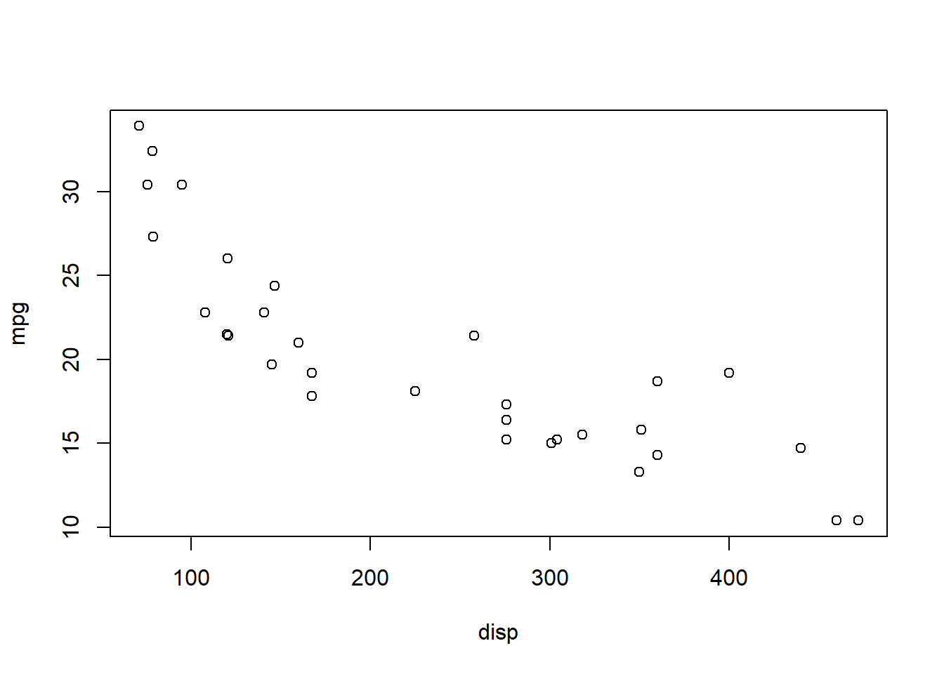
It appears fuel economy (measured as miles per gallon) generally declines with increasing engine size (measured as cylinder displacement volume).
Notice that \({\bf\textsf{R}}\) gave us a scatterplot even though we didn’t specify the graph type.
\({\bf\textsf{R}}\) saw that we were plotting a numeric vector against another numeric vector, for which the scatterplot is the default behavior for plot().
Let’s try another indepdendent variable:
plot(mpg ~ am, mtcars)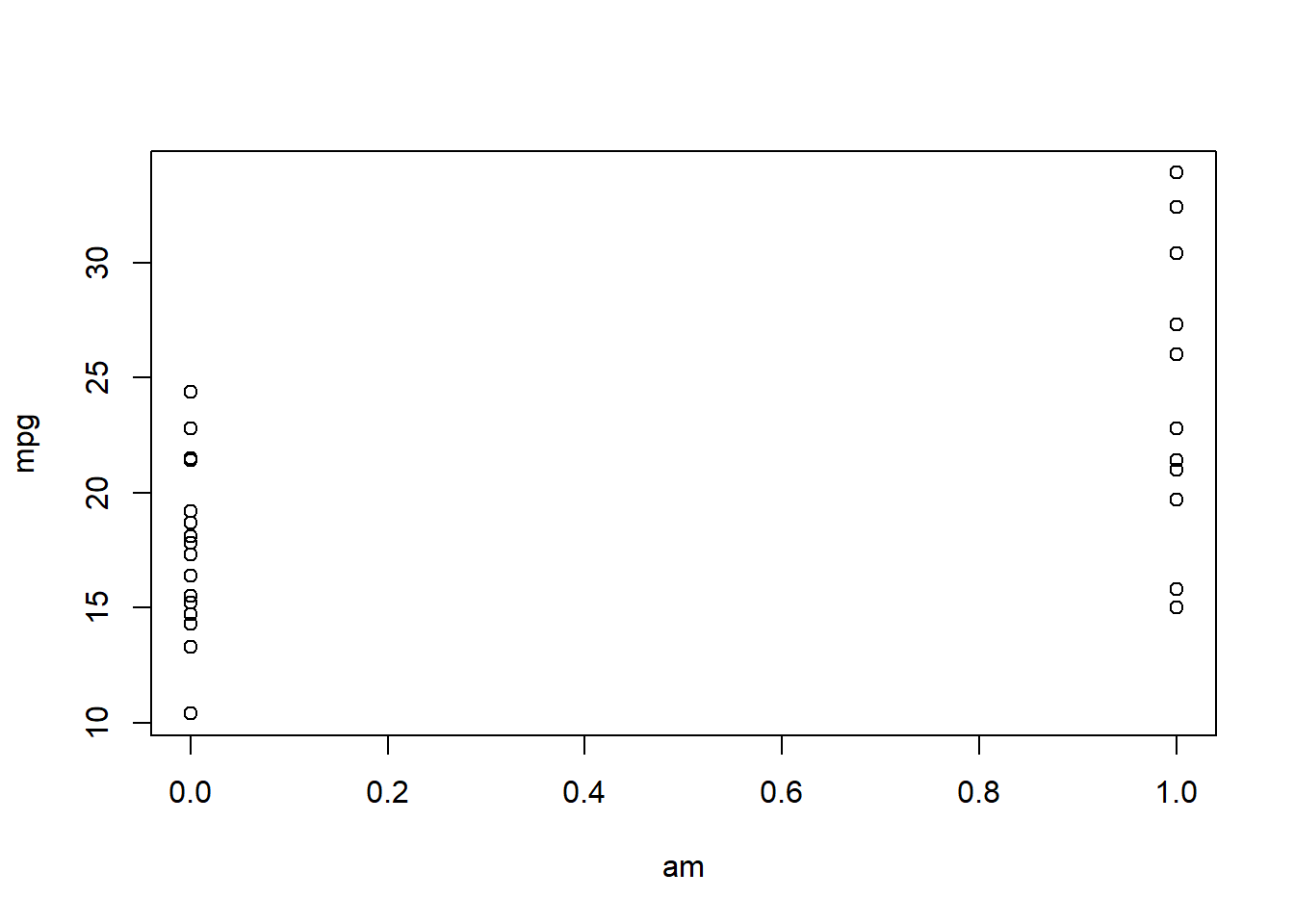
This is an awkward graph.
The X axis is a continuous scale, but the datapoints are stacked up at the edges, above 0 and 1.
\({\bf\textsf{R}}\) gave us a scatterplot because we gave it two numeric variables, but it appears likely that am should be classified as a categorical variable.
To learn more about these data, query the mtcars dataset:
?mtcars| mtcars {datasets} | R Documentation |
Motor Trend Car Road Tests
Description
The data was extracted from the 1974 Motor Trend US magazine, and comprises fuel consumption and 10 aspects of automobile design and performance for 32 automobiles (1973–74 models).
Usage
mtcars
Format
A data frame with 32 observations on 11 (numeric) variables.
| [, 1] | mpg | Miles/(US) gallon |
| [, 2] | cyl | Number of cylinders |
| [, 3] | disp | Displacement (cu.in.) |
| [, 4] | hp | Gross horsepower |
| [, 5] | drat | Rear axle ratio |
| [, 6] | wt | Weight (1000 lbs) |
| [, 7] | qsec | 1/4 mile time |
| [, 8] | vs | Engine (0 = V-shaped, 1 = straight) |
| [, 9] | am | Transmission (0 = automatic, 1 = manual) |
| [,10] | gear | Number of forward gears |
| [,11] | carb | Number of carburetors |
Source
Henderson and Velleman (1981), Building multiple regression models interactively. Biometrics, 37, 391–411.
Examples
require(graphics)
pairs(mtcars, main = "mtcars data", gap = 1/4)
coplot(mpg ~ disp | as.factor(cyl), data = mtcars,
       panel = panel.smooth, rows = 1)
## possibly more meaningful, e.g., for summary() or bivariate plots:
mtcars2 <- within(mtcars, {
   vs <- factor(vs, labels = c("V", "S"))
   am <- factor(am, labels = c("automatic", "manual"))
   cyl  <- ordered(cyl)
   gear <- ordered(gear)
   carb <- ordered(carb)
})
summary(mtcars2)
We can see that am refers to the transmission type–0 = automatic, 1 = manual–so in this case not only are the values categorical, but they don’t actually refer to the categories being expressed (recall cyl at least had categories called 4, 6, and 8 for the number of cylinders).
In addition to converting the vector class to a categorical type, we can also give the data meaningful names.
These three steps can be combined in what is called a dplyr pipe, and is rapidly being adopted by data scientists all over the internet.
The pipe operator, %>% was first introduced by the magrittr package (After years of wondering, the reference finally came to me in the shower one night).
It sort of reverses the right-to-left flow of the <- assigner and lets data “flow”, left to right, down through subsequent operations as if being poured down a pipe.
After the final operation, \({\bf\textsf{R}}\) returns what comes out of the pipe via <-.
There are many advantages that can mainly be summarized as, why use <- to create a whole bunch of objects along the way if we don’t care about the results of intermediary steps?
Pipes let us keep just the part we want.
Here’s an example of pouring mtcars through a pipe that performs three operations:
- Convert numeric column to factor with
as.factor - Change 0 and 1 to Automatic and Manual with
recode - Give a meaningful column name with
rename
mtcars <-
  mtcars %>%
    mutate(am = as.factor(am),
           am = recode(am, "0"="Automatic",
                           "1"="Manual")) %>%
      rename(transmission = am)
str(mtcars)
## 'data.frame': 32 obs. of 11 variables:
## $ mpg : num 21 21 22.8 21.4 18.7 18.1 14.3 24.4 22.8 19.2 ...
## $ cyl : Factor w/ 3 levels "4","6","8": 2 2 1 2 3 2 3 1 1 2 ...
## $ disp : num 160 160 108 258 360 ...
## $ hp : num 110 110 93 110 175 105 245 62 95 123 ...
## $ drat : num 3.9 3.9 3.85 3.08 3.15 2.76 3.21 3.69 3.92 3.92 ...
## $ wt : num 2.62 2.88 2.32 3.21 3.44 ...
## $ qsec : num 16.5 17 18.6 19.4 17 ...
## $ vs : Factor w/ 2 levels "0","1": 1 1 2 2 1 2 1 2 2 2 ...
## $ transmission: Factor w/ 2 levels "Automatic","Manual": 2 2 2 1 1 1 1 1 1 1 ...
## $ gear : Factor w/ 3 levels "3","4","5": 2 2 2 1 1 1 1 2 2 2 ...
## $ carb : Factor w/ 6 levels "1","2","3","4",..: 4 4 1 1 2 1 4 2 2 4 ...transmission is a categorical variable.
Let’s try plot() again:
plot(mpg ~ transmission, mtcars) 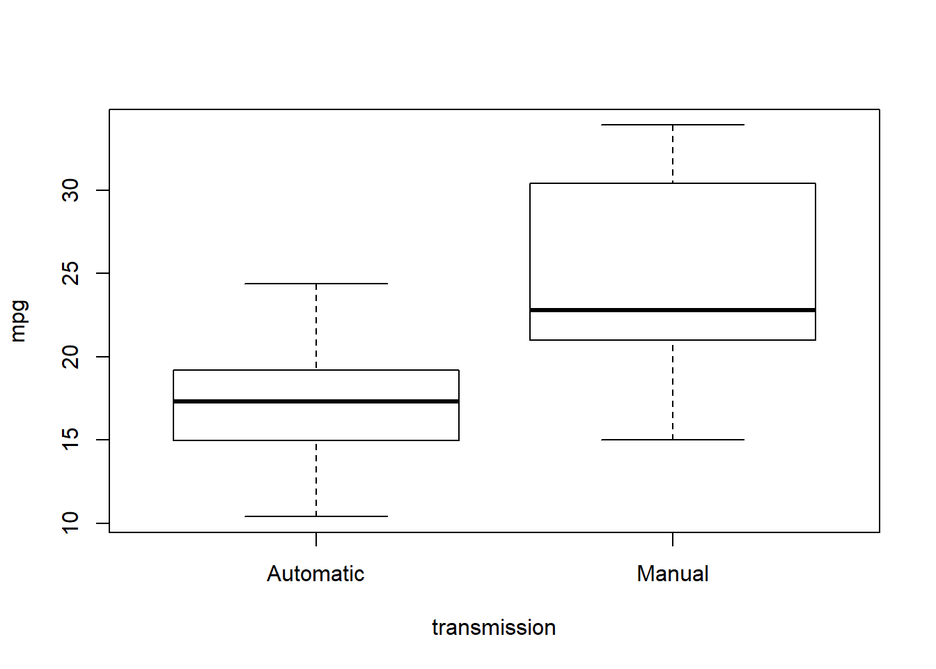
\({\bf\textsf{R}}\) assumes that when we give plot() a categorical independent variable, we want to see a boxplot, which is a good call.
Now, should we save our manipulated dataset? We saw arguments above for why we might not. However, in this case, I would argue that if this were my own dataset, there’s never a case when I’d want my data stored incorrectly, so it makes sense to save the corrected version:
getwd()
save(mtcars, file="./data/mtcars.Rdata")
# or
save(mtcars, file=file.choose())