Objectives
This lesson introduces ordination as a form of multivariate analysis, and covers several relevant vegan functions.
- Fitting an ordination object with
capscale - Graphing and interpreting the biplot
- Assessing the solution via eigenvalues and scree plots
- Extracting and interpreting site and species scores
- Understanding the impact of scaling on ordination results
Materials
Remember, If you aren’t familiar with multivariate data analysis, be sure to go over this introductory blog post.
About all you could ever want to know about ordination is available on Dr. Mike Palmer’s ordination webpage.1
Script
Video lecture
Walking through the script
Packages and data set-up
pacman::p_load(tidyverse, vegan)
data("varechem")
chem_d <- select(varechem, N:Mo)
as_tibble(chem_d)
## # A tibble: 24 x 11
## N P K Ca Mg S Al Fe Mn Zn Mo
## <dbl> <dbl> <dbl> <dbl> <dbl> <dbl> <dbl> <dbl> <dbl> <dbl> <dbl>
## 1 19.8 42.1 140. 519. 90 32.3 39 40.9 58.1 4.5 0.3
## 2 13.4 39.1 167. 357. 70.7 35.2 88.1 39 52.4 5.4 0.3
## 3 20.2 67.7 207. 973. 209. 58.1 138 35.4 32.1 16.8 0.8
## 4 20.6 60.8 234. 834 127. 40.7 15.4 4.4 132 10.7 0.2
## 5 23.8 54.5 181. 777 126. 39.5 24.2 3 50.1 6.6 0.3
## 6 22.8 40.9 171. 692. 151. 40.8 105. 17.6 43.6 9.1 0.4
## 7 26.6 36.7 171. 739. 94.9 33.8 20.7 2.5 77.6 7.4 0.3
## 8 24.2 31 138. 395. 45.3 27.1 74.2 9.8 24.4 5.2 0.3
## 9 29.8 73.5 260 749. 105. 42.5 17.9 2.4 107. 9.3 0.3
## 10 28.1 40.5 314. 541. 119. 60.2 330. 110. 61.7 9.1 0.5
## # ... with 14 more rowsFit a cluster diagram that we’ll end up using later:
chem_m <- vegdist(chem_d, method="euclidean")
chem_clust <- hclust(chem_m, method="average")
Fitting an ordination
A common ordination method is Principal Components Analysis, or PCA. All ordinations are based on an underlying distance matrix, and PCA is no different–it is based on the Euclidean distance measure. So while many ordination methods allow the user to specify the distance measure, when Euclidean is specified, the result is a PCA no matter what function produced it.
We use here vegan::capscale to perform our PCA because capscale offers the most flexibility for conducting a variety of ordinations in \({\bf\textsf{R}}\), even ones beyond what we’ll cover in this course.
The base stats package in \({\bf\textsf{R}}\) provides a few functions to conduct a PCA2, but they are limited to PCA specifically, and it is an objective of this course to introduce you to the vegan package.
capscale returns easy-to-interpret ordination results, including PCA if one sets the arguments correctly.
These settings dial back a lot of the full functionality of capscale, which is actually a flexible and powerful function.
Setting 1: Perform unconstrained ordination
capscale is designed to perform constrained ordinations aka direct gradient analysis.
I am not a fan of constrained ordinations and do not cover them here, but it is relevant because capscale uses formula notation Y ~ x in which community data \(\mathbb{Y}\) are fit against one or more constraining variables \(x\).
Because PCA is an unconstrained ordination we use Y ~ 1 and capscale forgets about constraints.
Setting 2: Perform Euclidean-based ordination
capscale can perform an ordination based on any of the \(15+\) distance measures listed in ?vegdist, and any you create yourself with designdist.
Since PCA is an ordination based on the Euclidean distance, we simply set method = "euc":
chem_pca <- capscale(chem_d ~ 1, method = "euc")Biplot
Dissimilarities are calculated in the distance matrix–if one wants to know exactly how similiar or dissimilar two sites are, one can look it up in the distance matrix. But matrices are unwieldy and a series of numbers does little to inform general questions about trends in the data across all the sites.
At its core, an ordination is a tool to identify where variation occurs in a multivariate dataset and reduce that variation into just a few composite variables that let one see the variation in fewer dimensions, ideally few enough that they fit on a screen or page. To see this, we need a way to graph the ordination.
The basic graph of an ordination result is called a biplot, but the bi part doesn’t refer to the two axes plotted, \(\textsf{x}\) and \(\textsf{y}\). Rather, biplot refers to the two components of information in the plot: site scores, and species scores.
- Site scores are the main result of the ordination.
- Numerically, site scores represent the location of each sampled point, or site, in ordination space.
- Conceptually, they represent the dissimilarity among the sites. Samples that are more similar are closer in the ordination, and samples that are more dissimilar are farther apart in the ordination.
- Because each row in a data frame of multivariate data represents one sample point, the length of the site scores equals that of the wide-format data frame.
- Species scores, when returned by an ordination,3, help one interpret which columns of the multivariate data correspond to variation in the ordination.
- They are called species scores because in conventional community ecology, the columns in multivariate datasets are the presence/absence or abundance in plant or animal species. But the columns can just as easily be trait data, etc.
- Scores further from the origin denote species with relatively greater contributions to overall variation.
- Especially at the periphery of an ordination–where most of the variation is apparent–sites closer to a species score likely tended to have a higher abundance of that species than, say, a site on the opposite side of the ordination.
By default, species scores are plotted as the column names, which is fairly easy to interpret, but site scores are plotted as row numbers.
While base stats does have a biplot function…
biplot(chem_pca, col=c("blue", "red")) 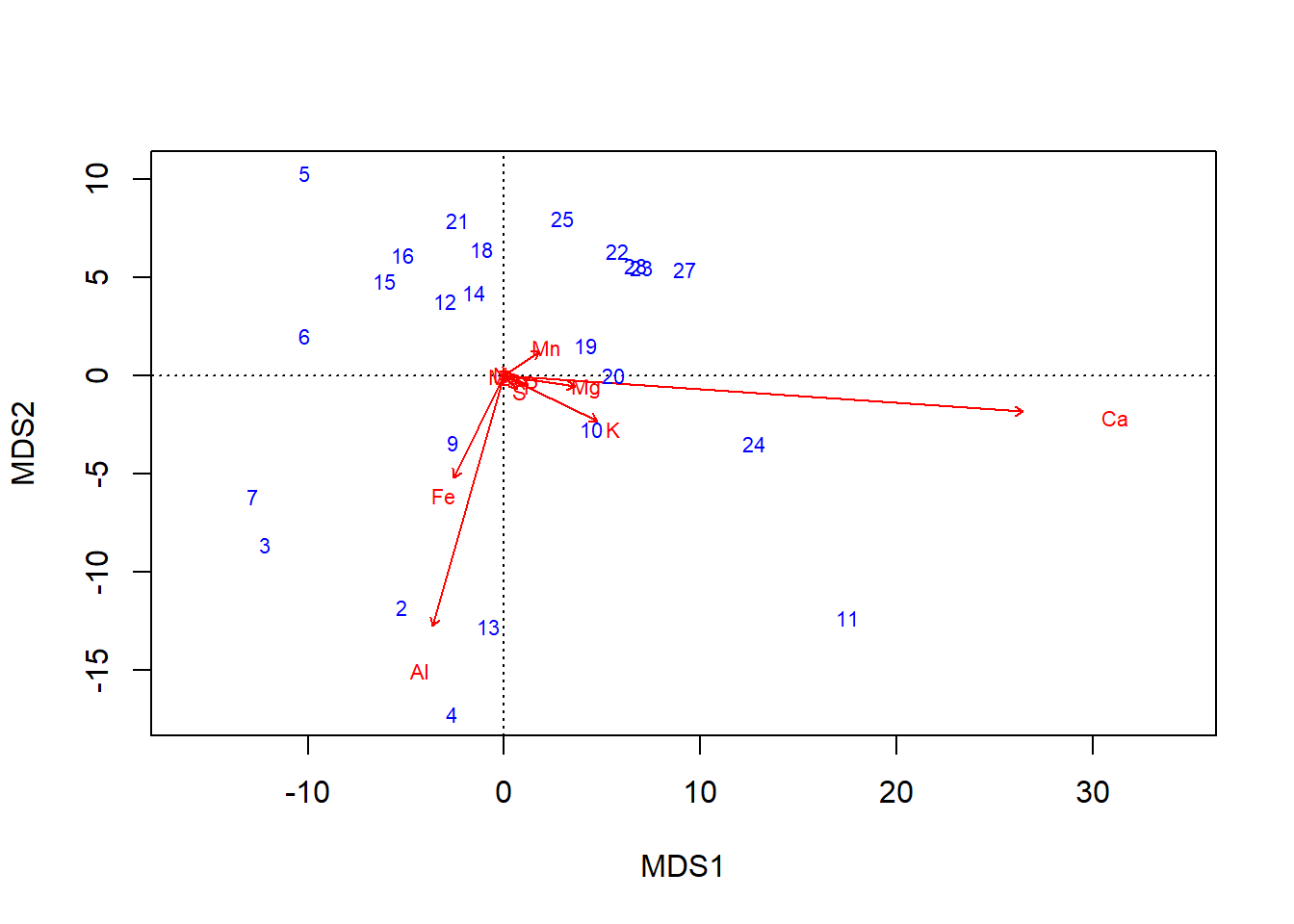
… graphics::plot can also handle vegan objects:
plot(chem_pca)
plot also offers more control, such as over whether one or both type of scores are shown…
plot(chem_pca, display = "sites")
plot(chem_pca, display = "species")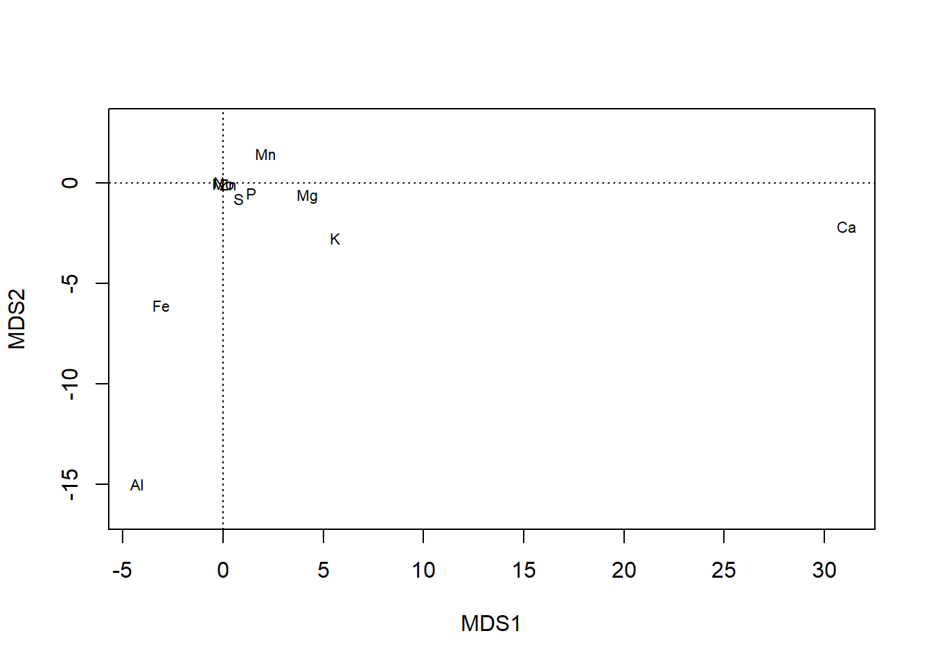
… and can even allow a blank plot (type='n') that can be filled with sequential calls to text:
plot(chem_pca, type="n") # Empty plot
  text(chem_pca, display = "species",
       col="red", cex=1.5)
  text(chem_pca, display = "sites",
       col="blue", cex=1.5)
Important note on axis labels
All axes labels are printed with \(\textsf{MDS}\), which stands for Multi-dimensional Scaling.
MDS refers to the general approach to unconstrained ordination employed by capscale, and \(\textsf{MDS}\) would be returned for any distance measure.
Many times, PCAs are plotted as \(\textsf{PCA2 x PCA1}\), and one might consider changing the axis labels to ensure readers remember you are reporting a PCA, even though as savvy vegan users we know an MDS fit with the Euclidean distance measure is a PCA.
Interpreting scores
Ordinations are about visualizing patterns in multivariate data, but two things are important for ordinations to be useful:
- Insight into what accounts for the patterns
- Confidence that the picture is meaningful
Both of these are addressed by analyzing the site and species scores, and both begin by retrieving them with vegan::scores and the display= argument:
Site scores (display = "sites"); note rownames as row numbers from original dataset:
scores(chem_pca, display = "sites", choices = c(1:10)) %>%
head %>% round(1) %>% pander::pander()| MDS1 | MDS2 | MDS3 | MDS4 | MDS5 | MDS6 | MDS7 | MDS8 | MDS9 | MDS10 | |
|---|---|---|---|---|---|---|---|---|---|---|
| 18 | -1.1 | 6.5 | 0.4 | 7.2 | 3.8 | 0.8 | 3.9 | -7.5 | 0.8 | -10.3 |
| 15 | -6.1 | 4.8 | -8.3 | 1.8 | 4.8 | 4.8 | 4.7 | -16.5 | 6.7 | 3.8 |
| 24 | 12.7 | -3.5 | 6.9 | -2.2 | 20.5 | -10.2 | 9.1 | 3.4 | -4.8 | 13.5 |
| 27 | 9.2 | 5.4 | -8.1 | 9.3 | -3.8 | -11 | -5.2 | -6.6 | 9.2 | 9.2 |
| 23 | 7 | 5.5 | 2.4 | 0.5 | 6.1 | 4.5 | 6.1 | 5.7 | -0.1 | -17.2 |
| 19 | 4.1 | 1.5 | 1.8 | -3.5 | 13.6 | -8.4 | -8.8 | -0.5 | 5.1 | -2.8 |
Species scores (display = "species"); note rownames as column names from original dataset:
scores(chem_pca, display = "species", choices = c(1:10)) %>%
round(2) %>% pander::pander() | MDS1 | MDS2 | MDS3 | MDS4 | MDS5 | MDS6 | MDS7 | MDS8 | MDS9 | MDS10 | |
|---|---|---|---|---|---|---|---|---|---|---|
| N | -0.19 | 0.07 | -0.06 | 0.25 | 0.03 | -0.05 | -0.21 | 0.59 | -0.08 | -0.02 |
| P | 1.41 | -0.49 | -0.59 | 0.08 | -0.23 | -0.35 | 0.94 | 0.15 | 0.12 | 0 |
| K | 5.59 | -2.72 | -5.42 | 0.12 | 0.48 | 0.85 | -0.04 | 0.01 | 0.03 | 0 |
| Ca | 31.1 | -2.15 | 1.36 | 0.02 | -0.4 | 0.08 | -0.02 | 0 | -0.01 | 0 |
| Mg | 4.22 | -0.63 | -0.27 | 0.19 | 2.9 | -0.96 | -0.08 | -0.01 | 0.06 | 0 |
| S | 0.79 | -0.78 | -0.74 | -0.24 | 0.32 | -0.23 | 0.3 | -0.1 | -0.36 | -0.04 |
| Al | -4.28 | -15.01 | 0.13 | -1.28 | -0.44 | -0.41 | -0.08 | 0.01 | 0.02 | 0 |
| Fe | -3.05 | -6.1 | 1.2 | 3.43 | 0.31 | 0.42 | 0.07 | -0.03 | -0.02 | 0 |
| Mn | 2.12 | 1.47 | -2.45 | 1.39 | -1.53 | -1.37 | -0.2 | -0.05 | 0.01 | 0 |
| Zn | 0.26 | -0.05 | -0.07 | -0.08 | 0.06 | -0.12 | 0.07 | 0.06 | -0.09 | 0.17 |
| Mo | -0.01 | -0.01 | 0 | -0.01 | 0 | -0.01 | 0.01 | 0 | -0.01 | 0 |
In metric ordinations such as those returned by capscale, there are \(n-1\) dimensions, with \(n=\) the number of species (columns). Only the first few are of importance, so we narrow it here to 10 via choices=.
Assessment
Since most ordinations are visualized in the two dimensions of a screen or page, the more variation explained by the first two axes of the ordination, the better a plot of that ordination is at showing the underlying patterns. Each additional axis explains additional variation, but marginally less each time: the first axis explains the most (but rarely a majority); the second axis a bit less, but more than the third; until all variation is explained by \(n-1\) axes, with \(n=\) the number of species (columns) in the data.
There are two general approaches to determining how well the first few axes represent the overall variation:
- Eigenvalues are a direct measure of how important an axis is to the overall solution. The larger the eigenvalue, the more important the axis.
- Proportion variance explained is intuitive.
capscaleresults show the % variance explained by each axis, and the cumulative variation explained by that axis and all those before it. Rule of thumb: \(70\%\) is a common cut-off. If \(70\%\) of cumulative variation can be explained in the first two axes–the ones shown in the graph–the ordination can be trusted. Note that even if it takes 3 axes to sum to \(70\%\), the ordination in general is pretty good, because most of the variation is still in axes \(1\)-\(2\).
As with so many other statistical functions, we use summary to see our PCA results:
summary(chem_pca)$cont %>%
  as.data.frame %>%
    round(2) %>%
pander::pander() | importance.MDS1 | importance.MDS2 | |
|---|---|---|
| Eigenvalue | 64044 | 16928 |
| Proportion Explained | 0.75 | 0.2 |
| Cumulative Proportion | 0.75 | 0.95 |
| importance.MDS3 | importance.MDS4 | |
|---|---|---|
| Eigenvalue | 2413 | 946.1 |
| Proportion Explained | 0.03 | 0.01 |
| Cumulative Proportion | 0.98 | 0.99 |
| importance.MDS5 | importance.MDS6 | |
|---|---|---|
| Eigenvalue | 704.4 | 248.3 |
| Proportion Explained | 0.01 | 0 |
| Cumulative Proportion | 1 | 1 |
| importance.MDS7 | importance.MDS8 | |
|---|---|---|
| Eigenvalue | 65.68 | 23.22 |
| Proportion Explained | 0 | 0 |
| Cumulative Proportion | 1 | 1 |
| importance.MDS9 | importance.MDS10 | |
|---|---|---|
| Eigenvalue | 9.95 | 1.92 |
| Proportion Explained | 0 | 0 |
| Cumulative Proportion | 1 | 1 |
| importance.MDS11 | |
|---|---|
| Eigenvalue | 0.02 |
| Proportion Explained | 0 |
| Cumulative Proportion | 1 |
Note the order of magnitude change from \(\textsf{MDS2}\) to \(\textsf{MDS3}\): The eigenvalues go from five digits to four, and the % explained goes from \(0.20\) to \(0.03\). Clearly we do not need to consider any axis after \(\textsf{MDS2}\), which suggests this is a robust solution for these data.
Scree plots are a great way to visualize how each additional axis contributes marginally more variation. As axes are added, the amount of remaining variation, or inertia, goes down. Obivously, a large number of axes eats up a lot of variation, but we want to see our first few axes perform well. This is depicted in the scree plot by steep slopes at first, then shallow slopes as the latter axes are plotted. One looks for a substantial inflection point where the slope changes noticebly, such as where one might find a pile of rubble, or scree, that rolled down a steep mountain slope but slowed down as the slope became more gentle:
screeplot(chem_pca, type="lines")
We see the slope get substantially shallower after \(\textsf{MDS2}\) and get dang near flat after \(\textsf{MDS3}\), which just shows what we found in the summary table above.
Ordination vs. clustering
Ordination projections and cluster diagrams are two ways to view the relationships in the distance matrix. While the cluster diagram might have the best fidelity in terms of representing the actual distances between pairs of sites, it is difficult to compare relative differences between more than two sites or see how groups relate to each other, because the information is conveyed by how high up the branch occurs. As two-dimensional projections of points arranged by an algorithm in multi-dimensional space, ordinations are often an abstraction of the distance matrix that better shows relative relationships. If we make sure the ordination is a good representation of the variation in the distance matrix, we can live with the abstraction of the projection.
While you will rarely do this, we can see how the relationships in the cluster diagram are arranged in the ordination.
This exercise also introduces the important group of ordi* functions vegan provides for showing groups and clusters in the ordination, which visualize the groups and gradients we test post-hoc for statistical correlations with the latent variable (and thus interpret as possible sources of variation in the multivariate data).
First, we use an old-school, base graphics way to put plots side-by-side.4
Then we use vegan::ordicluster to connect the site scores in the ordination chem_pca by the dendrogram stored in the cluster diagram object, chem_clust.
par(mgp=c(4, 1, 0),
    mar=c(6, 6, 1, 1),
     mfrow=c(1,2),
    las=1, cex.lab=1, cex.axis=1)
plot(chem_clust, las=1,
      labels=chem_d$name,
      xlab="Sample",
     ylab="Euclidean distance")
plot(chem_pca, display = "sites", las=1)
ordicluster(chem_pca, chem_clust)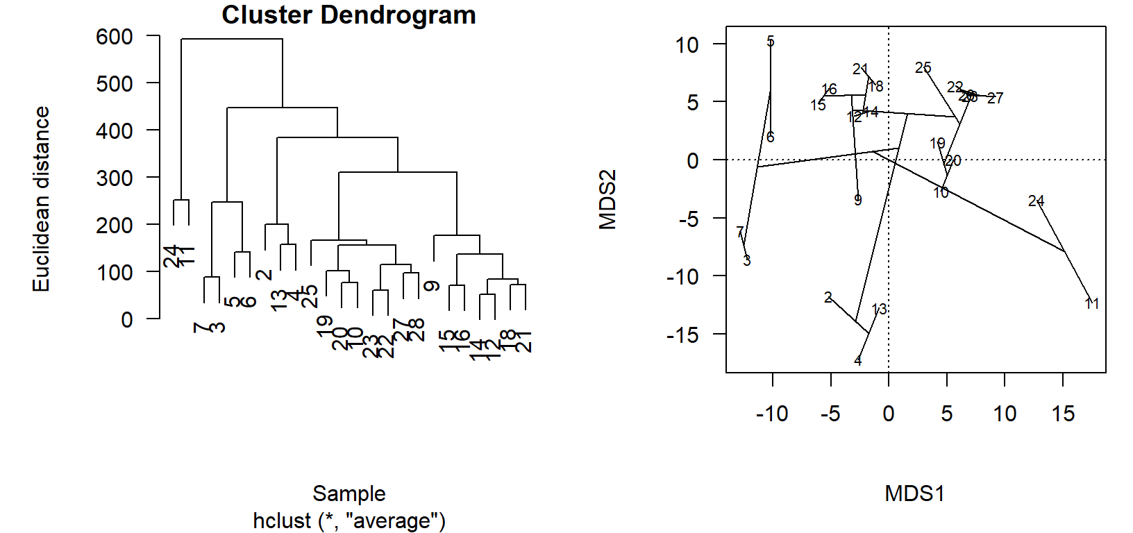
In the cluster diagram, we see that sites \(24\) and \(11\) are paired together but off on their own; this is apparent in the ordination projection, as well. Likewise sites \(2\), \(13\), and \(4\) share a branch in the dendrogram, and group closely together in the ordination.
The utility of the ordination comes in the visualization of very dissimilar sites, which are less obvious in the cluster diagram. Take, for example, how sites \(3\) and \(7\) are on the left of the primary axis of variation (\(\textsf{MDS1}\)), while \(24\) and \(11\) are on the far right. This is to be determined as these site groups to be maximally dissimilar, but the clusters appear side-by-side in the dendrogram! One must look up, and see thatalthough the clusters are printed side-by-side, they actually only connect at a very high level (large Euclidean distance, high dissimilarity).
Scaled data
We have applied scaling functions to our data a couple of times before, most recently prior to calculating the distance matrix for cluster analysis. Scaling data can have major implications on results, especially for multivariate analyses.
There are arguments for and against scaling, but for our purposes here, I generally advise scaling data prior to multivariate analysis. It has its greatest effect–and I would often argue, is most necessary–when the values across columns in the data occur on different scales.
Recall our initial ordination on unscaled data:
plot(chem_pca)
summary(chem_pca)$species %>%
  as.data.frame %>%
  select(MDS1) %>%
  round(2) %>%
t() %>% pander::pander() | N | P | K | Ca | Mg | S | Al | Fe | Mn | |
|---|---|---|---|---|---|---|---|---|---|
| MDS1 | -0.19 | 1.41 | 5.59 | 31.1 | 4.22 | 0.79 | -4.28 | -3.05 | 2.12 |
| Zn | Mo | |
|---|---|---|
| MDS1 | 0.26 | -0.01 |
The plot and primary axis scores indicate that the Calcium \(\text{Ca}\) gradient has the strongest influence on variation in the dataset (by an order of magnitude; \(31.1~vs.~5.59\). One might reasonably conclude, then, that calcium is the most important of the nutrients measured.
But let’s look back at the original data:
head(chem_d) %>% pander::pander() | N | P | K | Ca | Mg | S | Al | Fe | Mn | Zn | Mo | |
|---|---|---|---|---|---|---|---|---|---|---|---|
| 18 | 19.8 | 42.1 | 139.9 | 519.4 | 90 | 32.3 | 39 | 40.9 | 58.1 | 4.5 | 0.3 |
| 15 | 13.4 | 39.1 | 167.3 | 356.7 | 70.7 | 35.2 | 88.1 | 39 | 52.4 | 5.4 | 0.3 |
| 24 | 20.2 | 67.7 | 207.1 | 973.3 | 209.1 | 58.1 | 138 | 35.4 | 32.1 | 16.8 | 0.8 |
| 27 | 20.6 | 60.8 | 233.7 | 834 | 127.2 | 40.7 | 15.4 | 4.4 | 132 | 10.7 | 0.2 |
| 23 | 23.8 | 54.5 | 180.6 | 777 | 125.8 | 39.5 | 24.2 | 3 | 50.1 | 6.6 | 0.3 |
| 19 | 22.8 | 40.9 | 171.4 | 691.8 | 151.4 | 40.8 | 104.8 | 17.6 | 43.6 | 9.1 | 0.4 |
The \(\text{Ca}\) column has much greater values than most other columns: min \(\text{Ca} = 188.5\); max \(\text{N} = 33.1\), max \(\text{Mo} = 1.1\). Curiously, these lower-range elements cluster in the middle of the ordination. What if the apparent importance of calcium is simply an artefact of having the largest values, not the widest gradient of relative values, which is what the ordination is looking for?
Scale & fit
We can fit an ordination on scaled data, which preserves the relative relationships between values within columns but standardizes the range across all columns:
chem_s <- scale(chem_d)
chem_pca2 <- capscale(chem_s ~ 1, method = "euc")
plot(chem_pca2)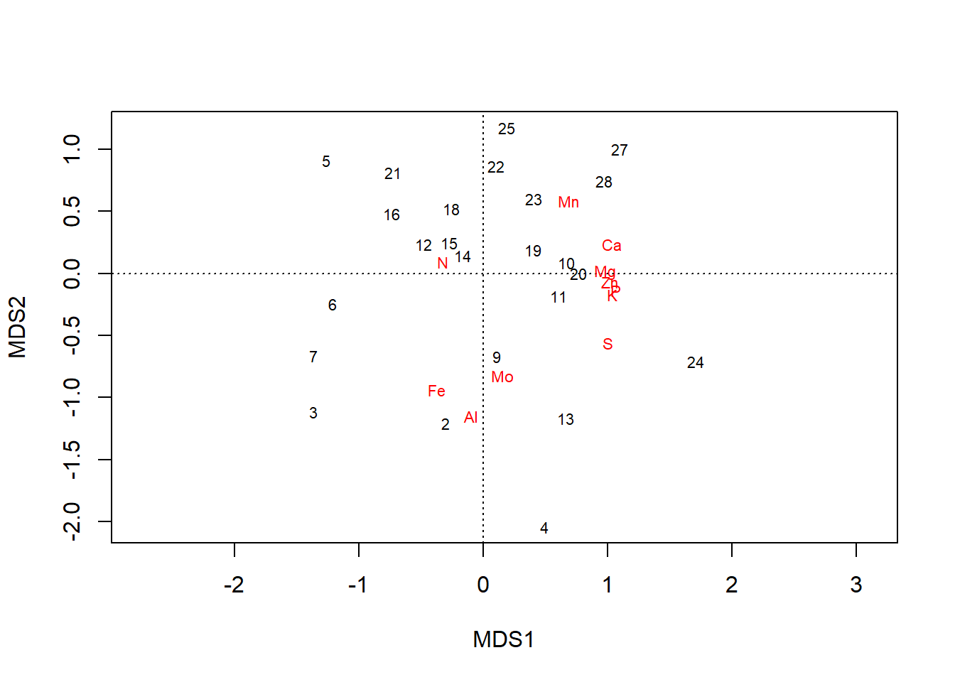
summary(chem_pca2)$species %>%
  as.data.frame %>%
  select(MDS1) %>%
  round(2) %>%
t() %>% pander::pander()| N | P | K | Ca | Mg | S | Al | Fe | Mn | Zn | Mo | |
|---|---|---|---|---|---|---|---|---|---|---|---|
| MDS1 | -0.33 | 1.07 | 1.04 | 1.03 | 0.98 | 1 | -0.1 | -0.37 | 0.68 | 1.02 | 0.15 |
In the plot, all elements are pulled away from the origin. Loadings along the first axis maintain their direction (e.g., \(\text{N}\) is still negative), and their relative positions, just across fewer orders of magnitude: \(\text{Ca} = 1.03\) and \(\text{Mo} = 0.15\). But now gradients in elements that simply occur in lower concentrations but are still important to plants–e.g., \(\text{P}\) & \(\text{K}\)–are revealed to have have important contributions to variation in the dataset, as well.
Eigenvalues
Scaling the data changes the performance of the PCA.
Firstly, the scale of eigenvalues is dialed back: \(\textsf{MDS1} = 4.9\), whereas before \(\textsf{MDS1}= 64044\). This new scale allows us to apply a second popular criterion for (metric) ordination assessment: axes with eigenvalues \(>1\) are important to variation, and the fewer axes it takes for eigenvalues \(<1\), the better the ordination represents the distance matrix.
summary(chem_pca2)$cont %>%
  as.data.frame %>%
.[1:6] %>% round(2) %>% pander::pander() | importance.MDS1 | importance.MDS2 | |
|---|---|---|
| Eigenvalue | 4.87 | 2.52 |
| Proportion Explained | 0.44 | 0.23 |
| Cumulative Proportion | 0.44 | 0.67 |
| importance.MDS3 | importance.MDS4 | |
|---|---|---|
| Eigenvalue | 1.08 | 0.88 |
| Proportion Explained | 0.1 | 0.08 |
| Cumulative Proportion | 0.77 | 0.85 |
| importance.MDS5 | importance.MDS6 | |
|---|---|---|
| Eigenvalue | 0.73 | 0.32 |
| Proportion Explained | 0.07 | 0.03 |
| Cumulative Proportion | 0.92 | 0.95 |
This criterion was not possible to apply to the unscaled data, but here we see the transition between \(\textsf{MDS3}\) and \(\textsf{MDS4}\). This is a more strict criterion than the \(70\%\) rule–this ordination result crosses that threshold earlier, between \(\textsf{MDS3}\) and \(\textsf{MDS4}\), and one might be tempted to round \(\textsf{MDS2}\) up.
Taken together, these statistics indicate the ordination is robust, with three axes accounting for a substantial amount of variation, and the third only containing \(10%\). The screeplot visualizes both criteria:
screeplot(chem_pca2, type="lines")
  abline(a=1, b=0, lty=2)
Note the substantial inflection at \(\textsf{MDS3}\).
Great power = great responsibility
If your brain is still on, you should be thinking, Wait, if it is good for an ordination to explain 70% cumulative variation in fewer axes, why is the scaled one better than the unscaled one, which explained 75% of variation in the first axis alone? And that would be a good question.
This is one of those ceteris paribus situations–assuming all else is equal–and in the unscaled data, all is not equal.
Calcium is weighted by the nature of the data, not the underlying process for which an explanation is sought through the collection of the data.
To make things equal, and assess the fit of the ordination fairly, all else must be equal, so we standardize the data to the same order of magnitude with scale.
It might not always be the best for your data, but my general advice is to scale data for multivariate analysis, especially when columns range across different orders of magnitude.
One soon learns that there are many choices at many junctures with multivariate analysis:
- which distance measure to use?
- Which
method=inhlcust? - How many clusters?
- scaled or unscaled data?
- 70% cumulative variation, or \(< 1\) eigenvalue?
\({\bf\textsf{R}}\) only gives an error if you coded something wrong. It won’t say that one should use scaled or unscaled data, or that the Canberra distance measure is more appropriate than Euclidean.5 Therefore, one cannot just quickly code an ordination and copy-paste the first graph that didn’t produce an error. One must scrutinize the results and ensure that the patterns revealed by the returned solution make sense for the study system. This takes practice and more reading and learning about multivariate stats than you get from Intro to \({\bf\textsf{R}}\).
Lots to learn there for sure but bear in mind he’s of a different school of thought on ordination than I am. He’s all about direct gradient analysis using versions of Canonical Correspondence Analysis in a software package called CANOCO, while I lean towards Metric Multidimensional Scaling, obviously in \({\bf\textsf{R}}\). But the basic principles are the same.↩
These include
princompandprcomp↩Species scores are calculated after-the-fact and are therefore not necessarily returned by default from some vegan functions.↩
When running this script yourself, you’ll probably want to use the
x11()call included in the script, or at least the ‘zoom’ button in \({\bf\textsf{R}}\) studio. ↩There are, of course, functions in vegan to compare their fit.↩