Objective
Multivariate data are different than what we’ve used so far, and so multivariate analyses are different, as well. This post introduces these differences ahead of the lessons in multivariate analyses.
Multivariate data
The primary difference between multivariate and univariate data is the number of response variables. All analyses we’ve applied so far have been univariate: regardless of the number of predictor variables, there have only been one response variable, \(y\).
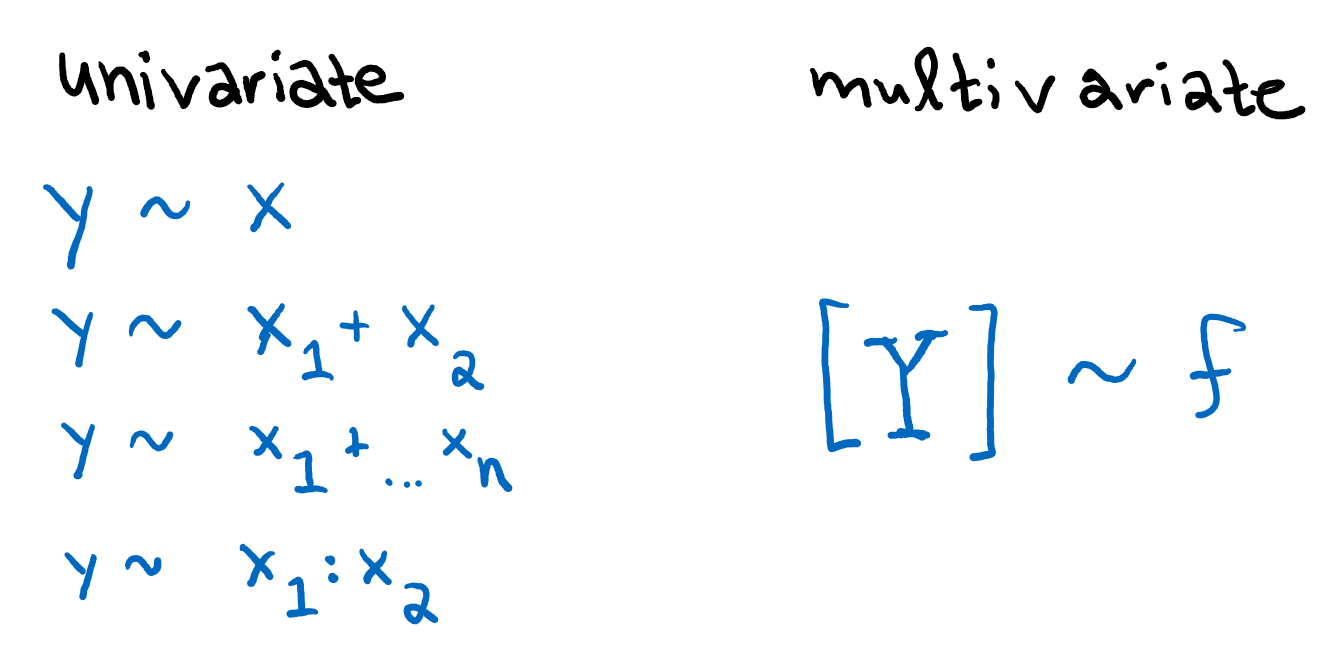
Multivariate data, as the term suggests, includes multiple response variables, which I simply refer to here as \(\mathbb{Y}\).
Multivariate analyses
Finding patterns
This is a very simple description of how the multivariate analyses we learn here generally work, with particular reference to how they differ from the univariate analyses we’ve learned. I highly suggest reading more in Greenacre & Primicero’s online book, Multivariate Analysis of Ecological Data1
Most multivariate analyses first seek to describe patterns of variation within the data–how the individually-observed samples (rows in the data frame) relate to one another based on the values of the multiple variables for which data were collected from each observation (columns in the data frame).
The distance matrix
The relationships between pairs of observations are stored in a distance matrix. These are calculated based on a variety of metrics called distance measures. The simplest is the Euclidean distance, which gives a straight-line distance between two observations in multivariate space–the more similar the points are based on the data in the columns, the smaller the Euclidean distance. Conversely, the more dissimilar the points are, the greater their Euclidean distance. This is the basis of a common multivariate analysis, Principal Components Analysis, or PCA.
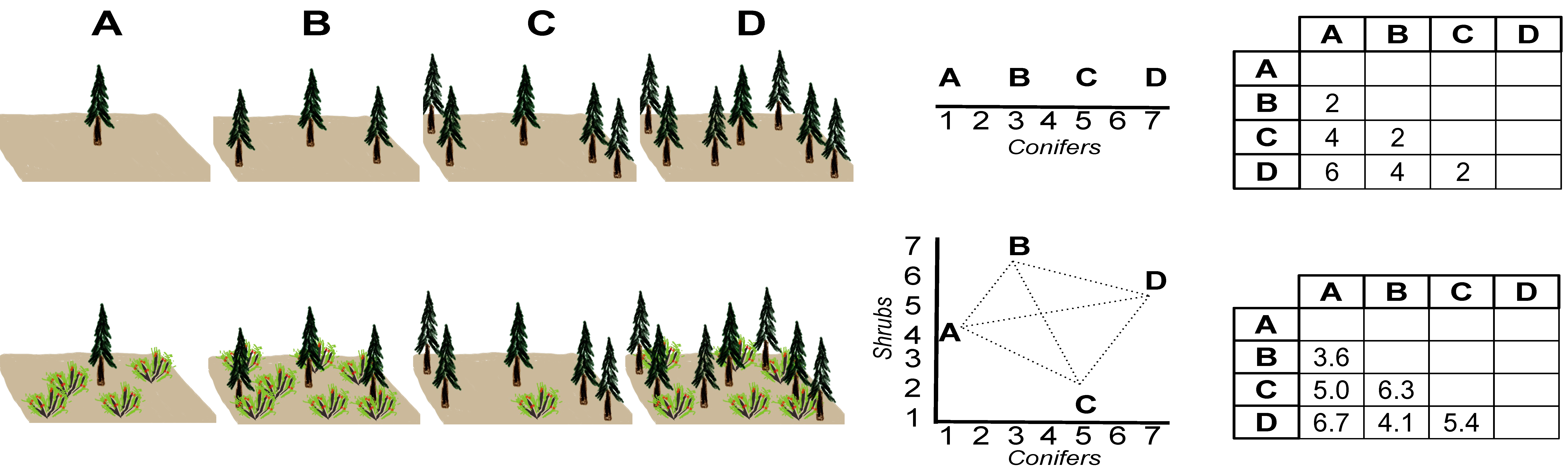
The figure below illustrates how Euclidean distances represent dissimilarity among two sites based first on the abundance of one species, conifers, and then on a two-species community comprised of both conifers and shrubs. Ranking the sites in the order of species abundance is essentially a (very simple) ordination, and the straight-line distances between them represent the Euclidean distances in the matrix.
Ordination
Ordination algorithms essentially perform this operation, but in reverse. It is difficult to graph more than two dimensions, but the straight-line distances can still be calculated in multiple dimensions. The ordination rotates the multi-dimensional point cloud such that the first two axes–the ones we can easily graph–represent the widest range of variation. The two-dimensional points we see are a projection of the multi-dimensional point cloud, as if a light were shined through it and the site scores we see in a graph are shadows on the wall.
Other measures have more complicated formulae that take into account, for example, the relative value of an observation within the range of the other observations. These are frequently used in analysis of data on ecological communities. Bray-Curtis dissimilarity is a frequent distance measure for such data. For lots more about ordination and ecological data, I highly recommend Chapter 10 in Kindt & Coe’s book, Tree Diversity Analysis.
Plots for multivariate data attempt to show the viewer the relationships stored in the distance matrix. This is often complicated, as the distance matrix is a numerical representation of multi-dimensional space–\(n-1\) dimensions, when \(n=\) the number of columns in the data frame–which is tough to depict on a two-dimensional screen or page. Options include cluster diagrams and the projections of the first two axes of ordinations, which are calculated to represent the majority of variation in the multivariate space.
The latent variable
Sometimes simple descriptions of patterns within multivariate data are sufficient, and there is no need for predictor variables, as one always has in a univariate analysis. In fact, most of the multivariate analyses we use here do not directly test predictor variables, even when we use additional information to determine what might account for the patterns in the data identified by the multivariate analysis.
While these additional data would function as predictor variables in a univariate analysis, our multivariate analyses test for a correlation between these variables and what is called a latent variable: the unknown driver of variation in the multivariate data.
post-hoc statistical tests
Because most of our statistical tests are post-hoc, testing only after-the-fact for a correlation between our known variables and the unknown latent variable described by the multivariate analysis, it is important not to assume too much in the way of causation. We should limit our interpretation of such results to descriptions of associations between environmental or management variables and patterns in the multivariate data. We must not go so far as to say these groups or gradients are drivers of the observed patterns.
Unfortunately the URL for the great website that hosted this book didn’t work for me, but the entire book is avialable on Google Books.↩