Objective
Step up your \({\bf\textsf{R}}\) markdown game by creating polished documents:
- Adding in-text citations and a bibliography that are compiled and formatted while knitting
- Hide code chunks from main body of text but include at end as an appendix
- Knit
.Rmd\(\rightarrow\).htmlfor sharing online
Materials
How-to video
Template & example files
A template to get started on Mini-report #1 for class.
The GitHub folder also includes two different .csl files and a .bib file used by the template.
Save all three to the same local folder on your machine. I suggest adding a folder to keep everything you need for a document together, in a structure that would look something like this:
R
│
└─── data
│
└─── script
       |
       └─── MiniReport1
Add a bibliography
Adding a bibliography to an .Rmd file requires at least two files.
It is easiest if they are in the same folder as the .Rmd file.
The yaml header
Every .Rmd file we’ve made has started with a yaml header:
---
  title:
  author:
  date:
---
Adding a bibliography requires two additional fields:
---
  title:
  author:
  date:
  csl:
  bibliography:
---
The .csl file
CSL stands for Citation Style Language, and the .csl file is what tells the knitting process what the in-text citations and bibliography should look like.
One usually starts by finding pre-existing .csl files and just saving them in the appropriate folder.
If something about the style it creates isn’t quite right, either find a different one or edit it yourself.
There are a ton of different styles. You’re probably familiar with the major types of bibliography styles: Modern Language Association, or MLA; American Pyschological Association, or APA; Harvard, Chicago, Vancouver, etc. etc.
Within each major group of styles, journals often have specific formats. Take, for example, this entry in the standard APA author-date format:
Sidoli, M. (1996). Farting as a defence against unspeakable dread. Journal of Analytical Psychology, 41(2), 165-178.
Journals published by the Ecological Society of America require this specific format:
Sidoli, M. 1996. Farting as a defence against unspeakable dread. Journal of Analytical Psychology 41:165–178.
But a Elsevier journal that used the author-date format would require different specifics:
Sidoli, M., 1996. Farting as a defence against unspeakable dread. Journal of Analytical Psychology 41, 165–178.
Switching back and forth between styles is a major pain, a giant waste of time, and a great way to fill your paper up with mistakes.
Using .csl files makes it a lot easier.
The .bib file
Style isn’t everything–now we need content.
The raw information that the .csl is going to make pretty for us is stored in a basic format known as BibTeX with file extention .bib.
BibTeX was originally designed to support bibliographic management within the \(\TeX\) typesetting system, but it has broader use for us here, as well.
Entries look like so:
@article{sidoli1996,
  title={Farting as a defence against unspeakable dread},
  author={Sidoli, Mara},
  journal={Journal of Analytical Psychology},
  volume={41},
  number={2},
  pages={165--178},
  year={1996}
}
Compile new
To create a .bib file in \({\bf\textsf{R}}\) studio, open a new plain ol’ text .txt file and simply save it with the .bib extension.
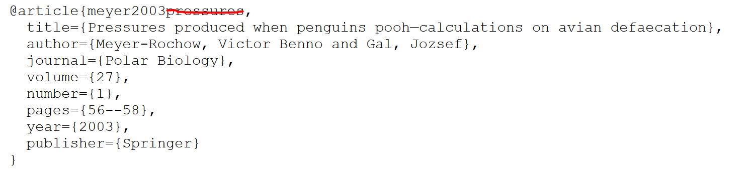
Google Scholar provides BibTeX-formatted reference information for each entry. Just click on the quote marks…
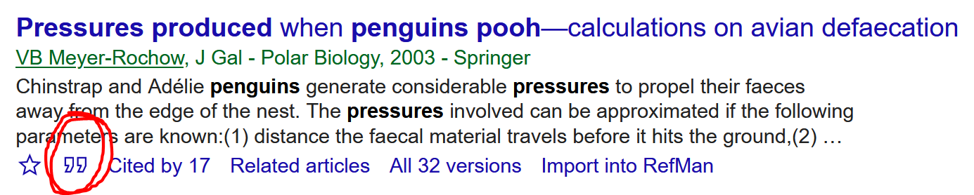
…select BibTeX…

…then just copy the text and paste into the .bib file:
Create from zotero
Most citation managers also accommodate BibTeX format; some even specialize in it.
I exclusively use zotero for reference management,1 because it facilitates importing .pdf files into the library; it efficiently extracts citation info so one doesn’t have to manually enter hardly anything at all, and it easily exports .bib files (the BetterBibTeX zotero add-on is a life-saver).
Just right-click on a zotero collection (folder) to export all entries therein as a bibliography in BibTeX format to the appropriate folder.
Add script appendix
Moving script from individual chunks throughout the document into a single chunk at the end of the document is simple. This is a great way to focus your document on the text and results but still share the details of how you got those results with your readers (I nearly always do this when I publish papers).
There are really just two steps:
- Hide code chunks from being shown where they occur in the document with code chunk option
echo=FALSE.
- Either put it in each code chunk,
- or set a document-level option for all chunks with
```{r setup, echo=FALSE, message=FALSE}
knitr::opts_chunk$set(message = FALSE,  warning=FALSE, echo=FALSE)
```- Make sure your
.Rmdfile ends like this (# Bibliographyoptional, of course):
# Script

```{r ref.label=knitr::all_labels( ), echo=TRUE,eval=FALSE}
```

# References cited
Knit to .html
An easy alternative to creating Word documents that does not require additional software is knitting to .html files.
These are easily viewed right in \({\bf\textsf{R}}\) studio’s Viewer pane, and are easily shared online.
.html files from .Rmd offer a lot more formatting options.
Remember, this whole blog was created by knitting .Rmd \(\rightarrow\) .html and uploading to GitHub.
But you don’t need a website to share yours.
Read all about HTML output from \({\bf\textsf{R}}\) markdown here.
Publishing
Documents can be posted online and shared via a unique URL right from \({\bf\textsf{R}}\) studio.
Once a .html file is knit locally, a Publish button appears in the upper right corner of the Viewer pane.
If one has a free acount on Rpubs, one can easily publish and share with just a few clicks.
Alternative formats
\({\bf\textsf{R}}\) Markdown users have the most control over formatting when knitting to .pdf, but that requires having \(\LaTeX\) installed on one’s computer.
Knitting to .html is a good balance between having control over appearance without additional software.
Knitting to .docx is the most limiting, although there are ways for users to develop their own templates for a bit more control over Word document format.2
There are many format options, called themes, available to customize the appearance of your knitted document.
To see the 14 pre-loaded themes, run
rmarkdown:::themes()## [1] "default" "cerulean" "journal" "flatly" "darkly" "readable"
## [7] "spacelab" "united" "cosmo" "lumen" "paper" "sandstone"
## [13] "simplex" "yeti"Even more themes are available from other packages, such as rmdformats, tufte, and my personal favorite, tint.
See visual examples of each here.
To use a theme, simply specify the theme (and any options, if available) in the yaml header:
---
  title:
  author:
  date:
  csl:
  bibliography:
  output:
    html_document:
      theme: journal
---

---
output:
   tufte::tufte_html:
    tufte_variant: "envisioned"
---
Once
.bibfiles are out of zotero and I need to edit them, I rely on JabRef.↩From what I can tell, this approach should afford one enough control over the output to make knitting to Word a viable option for collaboration, thesis-writing, and journal article creation.↩