Materials
Data
This lesson uses those same data on arrests around athletics venues in Cleveland, Ohio:1
Script
Video lecture
Walking through the script
Packages & data
Two external packages are required, but I recommend installing them but not loading them into the session.
They either contain functions that conflict with tidyverse functions, or automatically load up other packages that have conflicts.
Therefore, install them and refer to functions using the package::function convention.
Remember, only install them to a given machine once. Bad idea to constantly re-install packages already installed. And never put a call to install.packages in an .Rmd file.
install.packages(c("car", "lme4"))And we always need tidyverse!
pacman::p_load(tidyverse)We use the same data as in Lesson 9, the Cleveland crime data:
clev_d <- read_csv("./data/AllClevelandCrimeData.csv")clev_d <-
clev_d %>%
mutate(GameDay = recode(GameDay, "0" = "No",
"1" = "Yes")) %>%
select(GameDay, Venue)Analyzing count data
Recall the central research question: Are more arrests made on days with games at the two professional athletics facilities in Cleveland, Ohio?
Visualize with a bar chart…
ggplot(clev_d) + theme_bw(16) +
  geom_bar(aes(x=GameDay),
           stat="count")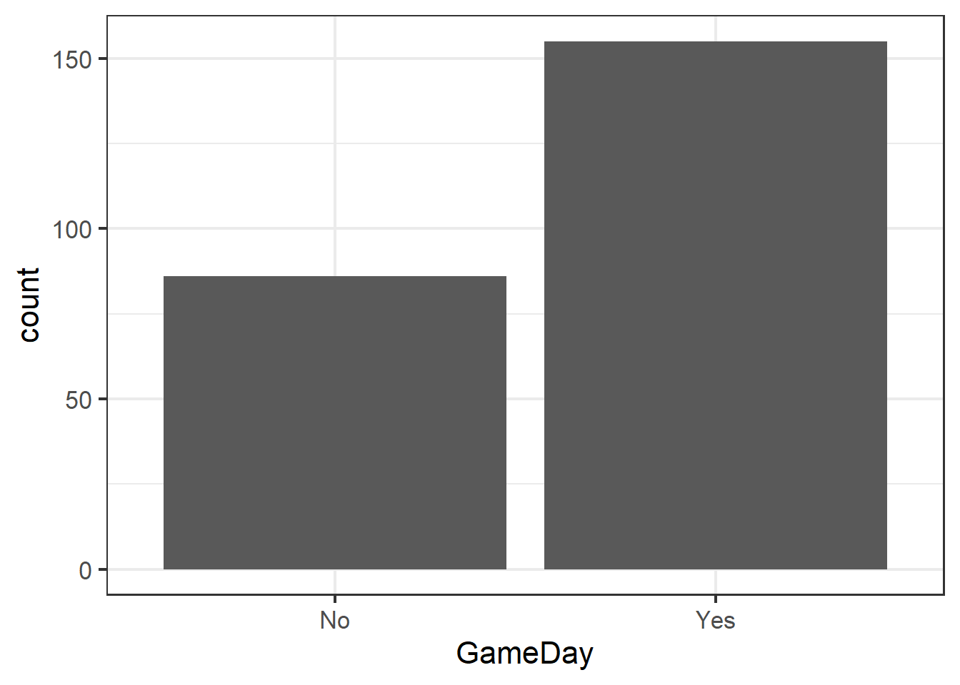
… generate a summary table to create the data to test…
GD <- clev_d %>%
        group_by(GameDay) %>%
          summarize(charges=n())
GD
## # A tibble: 2 x 2
## GameDay charges
## <chr> <int>
## 1 No 86
## 2 Yes 155Fitting a GLM
… and test with a generalized linear model, or GLM. GLMs are what we use to conduct linear regressions on non-continuous data like counts and probabilities, or even continuous data that don’t fit a normal distribution. GLMs assume the data fit non-Gaussian distributions; since there are many, we must specify which one we want the model to use.
The family= argument is required to tell glm() which distribution we want to use.
It includes an optional link= argument.
Link functions are not optional, but each family in \({\bf\textsf{R}}\) has a default.
Link functions are applied to the response variable, which because it is not normally distributed, requires a transformation to link it to the math that drives the general linear regression.
That’s why these are called generalized linear models–they use math to connect data that follow non-normal distributions to generally fit a linear regression.
Choosing appropriate options for family= and link= are beyond the scope of Intro to \({\bf\textsf{R}}\), but Poisson is a common distribution for count data, and we’ll use it here:
glm_gd <- glm(charges ~ GameDay, GD,
              family=poisson(link = "identity"))
Evaluating glm objects is similar to lm objects, but the results are a bit different due to differences in the underlying math.
The main difference is that instead of the typical \(t\) test based on a \(t\) distribution or ANOVA based on the \(F\) distribution, many GLM functions in \({\bf\textsf{R}}\) conduct an Analysis of Deviance that basically determines statically whether the ratio of the counts deviates from a null hypothesis of 50:50.
For example, if there were 100 arrests and game day had no effect, we’d expect about 50 to have occurred on game days, and 50 on days without games. The Analysis of Deviance tests the degree to which the observed data deviate from 50/50.
Because there is a little more/different math involved in the Analysis of Deviance than an ANOVA, there are more ways to get there. Thus there are different test statistic options, and various ways to code them in \({\bf\textsf{R}}\).
A few examples include:
summary(glm_gd)##
## Call:
## glm(formula = charges ~ GameDay, family = poisson(link = "identity"),
## data = GD)
##
## Deviance Residuals:
## [1] 0 0
##
## Coefficients:
## Estimate Std. Error z value Pr(>|z|)
## (Intercept) 86.000 9.274 9.274 < 2e-16 ***
## GameDayYes 69.000 15.524 4.445 8.8e-06 ***
## ---
## Signif. codes: 0 '***' 0.001 '**' 0.01 '*' 0.05 '.' 0.1 ' ' 1
##
## (Dispersion parameter for poisson family taken to be 1)
##
## Null deviance: 2.0034e+01 on 1 degrees of freedom
## Residual deviance: 9.7700e-15 on 0 degrees of freedom
## AIC: 17.177
##
## Number of Fisher Scoring iterations: 2This is fairly familiar output: the structure is the same, but instead of a \(t\) statistic like summary() on an lm object, the summary of a glm object returns a standardized z statistic.
Like the summary of lm objects, we can identify parts of our data in the coefficients of the glm object.
Recall how lm analyzes factors by assigning the first level as the intercept \(\beta_0\) and estimates the slope \(\beta_1\) as the difference between the intercept and another factor level.
Here, \(\beta_0 =86\), and since \(155-86=69\), \(\beta_1=69\).
Let’s try another function to evaluate regression objects:
anova(glm_gd)## Analysis of Deviance Table
##
## Model: poisson, link: identity
##
## Response: charges
##
## Terms added sequentially (first to last)
##
##
## Df Deviance Resid. Df Resid. Dev
## NULL 1 20.034
## GameDay 1 20.034 0 0.000The structure of this table is familiar but it is missing an important component: we don’t get a \(P\) value denoting the significance of the GameDay term.
This is because there are several options in how to perform the Analysis of Deviance, and anova needs to be told how to do it via the test= argument:
anova(glm_gd, test = "Chisq") ## Analysis of Deviance Table
##
## Model: poisson, link: identity
##
## Response: charges
##
## Terms added sequentially (first to last)
##
##
## Df Deviance Resid. Df Resid. Dev Pr(>Chi)
## NULL 1 20.034
## GameDay 1 20.034 0 0.000 7.606e-06 ***
## ---
## Signif. codes: 0 '***' 0.001 '**' 0.01 '*' 0.05 '.' 0.1 ' ' 1This table confirms that the increase in arrests on game days is statistically significant.
This is based on a \(\chi^2\) statistic, instead of the \(z\) score in summary, similar to how with an lm object, summary returns a \(t\) statistic and anova returns an \(F\) statistic.
They are just based on different math.
The car package
At this point we need to meet the Companion to Applied Regression package, car. car contains a number of helpful functions (I’ve only begun to scratch the surface), some of which are discussed more in Analysis of Ecosystems.
Here we focus on the Anova function.
It extends the functionality of base stats::anova.
For example, when it detects a glm object, it defaults to an Analysis of Deviance based on a \(\chi^2\) statistic; it doesn’t need us to tell it:2
car::Anova(glm_gd) ## Analysis of Deviance Table (Type II tests)
##
## Response: charges
## LR Chisq Df Pr(>Chisq)
## GameDay 20.034 1 7.606e-06 ***
## ---
## Signif. codes: 0 '***' 0.001 '**' 0.01 '*' 0.05 '.' 0.1 ' ' 1Analyzing non-independent data
One of the assumptions of statistical analysis is that the observations in a dataset are independent–the value of a given data point doesn’t have anything to do with the value of another data point any more than any other data point. Researchers often satisfy this assumption by randomly assigning treatment groups across multiple replicated plots and assuring samples are collected at sufficient distances to avoid spatial autocorrelation.
Such randomization is often not an option for observational studies, and many hierarchical sampling designs intentionally build in spatial dependence to determine to account for or even test for spatial patterns. Data from such designs often do not meet the assumption of independence and are instead often examples of pseudoreplication–when the number of observational units (samples) is greater than the number of experimental units (true replicates).3
Take, for example, a study with 5 plots from which 3 samples each have been collected.
The number of observational units = 15, but \(n \neq 15\).
Instead, \(n=5\), the number of experimental units.
One cannot run a basic statistical test like lm or glm on the whole dataset, because the model will assume \(n=15\) and \(df = 14\); this artifically high statistical power will return a problematic \(P\) value that is lower than would be returned by the actual statistical power of five true replicates (\(df=4\)).
Our present data set poses this problem. Arrests in the dataset are not independent, as there are two main centers around the venues from which arrests were made. There are differences in the venues that are not part of our hypotheses. For example, the venues have different capacities, and since they have different sports in different seasons, they might have different types of fans. For these reasons and likely others, arrests made at one venue cannot be assumed to be independent of one another.
 ggplot(clev_d) + theme_bw(16) +
   geom_bar(aes(x=GameDay,
                fill=Venue),
            stat="count",
            position = position_dodge2())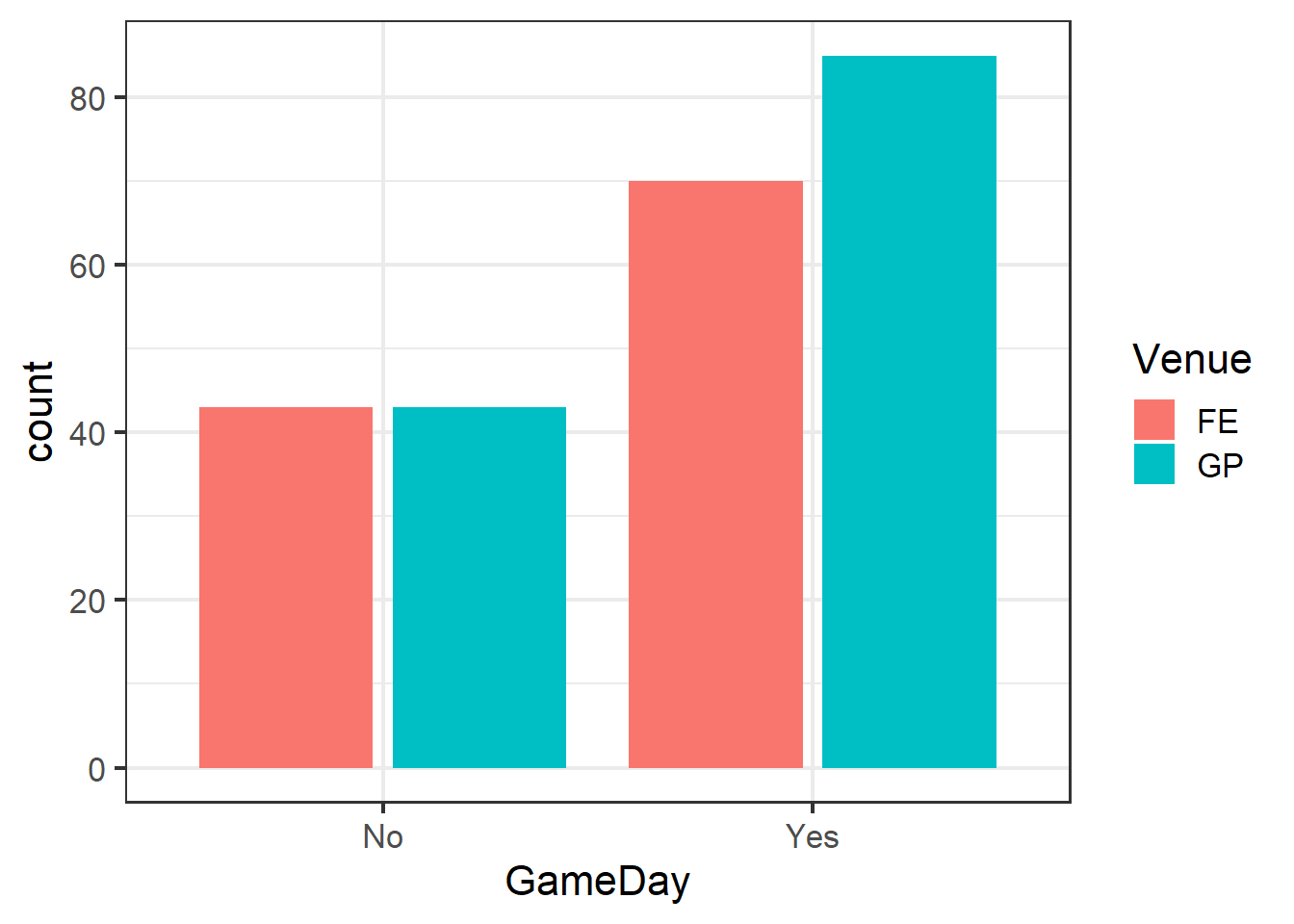
Note the use of position_dodge2 to create side-by-side, rather than stacked, bars.
Indeed, even though both venues did increase as we expected, the degree of their responses differed across the venues.
Among several possible ways to handle this situation, the primary two are:
- Calculate summary statistics for each experimental unit from the sub-sampled observations
- Use a model that can properly account for the nested sampling scheme (i.e., and not assume a simple variance structure in which variance is pooled among all observations, but calculate unique variance estimates for each discrete experimental unit)
Option (1) is the easiest and facilitates a basic (g)lm with the appropriate degrees of freedom.
However, option (1) has drawbacks: in a study with a lot of plots, it can be demoralizing to see all of the effort put into collecting multiple sub-samples per plot essentially erased by compositing them into a summary statistic.
Option (2) allows us to retain not only the sample size provided by the sub-sampled observations, but also the information about the variance structure within each experimental unit.
There are a few examples of statistical models, all based on the basic linear regression/ANOVA framework we learned before. One option is to include a blocking factor in the ANOVA model: ?aov gives us the example of aov(yield ~ N*P*K + Error(block), npk).
In many cases, the better option is to use a mixed-effect model. By mixed-effect, we mean that the model will include terms for the independent predictor variables we are interested in (fixed effects) in addition to independent variables we know might contribute to variation but we don’t have a hypothesis for. We add these variables to the model as random effects, which allows the model to control for them, rather than test them.
Note that this assumption of independence is a different issue than having continuous and/or normally-distributed data. Thus, mixed-effect models are available for cases in which we’d fit a linear regression model to continous data that follow a normal distribution, and cases in which we’d turn to a generalized linear model.
Several packages fit mixed-effect models in \({\bf\textsf{R}}\). I use a very popular package called lme4; you can read all about it here.
Fitting a GLMM
GLMM stands for Generalized Linear Mixed-Effect regression Model.
We will fit one with lme4::glmer.
But first, let’s look at the summary count table of arrests by game day or not across venues:
GD_v <- clev_d %>%
          group_by(Venue, GameDay) %>%
            summarize(charges=n()) %>%
          ungroup
GD_v
## # A tibble: 4 x 3
## Venue GameDay charges
## <fct> <chr> <int>
## 1 FE No 43
## 2 FE Yes 70
## 3 GP No 43
## 4 GP Yes 85lme4 functions follow the same Y ~ X formula notation as (g)lm.
We simply add the random effect in parentheses.
It has two components: a term to modify the slope of the regression lines, and a term to modify the intercept of the regression lines, separated by the vertical bar, |.
Recall from our lesson on multiple regression and interaction terms that it is pretty serious business to start modelling different slopes, so in this case, we’ll leave it alone by entering \(1\) on the left of the bar.
Recall also that there are many reasons why we might allow the intercept to vary among groups. If we have a hypothesis for how a variable that might cause different intercepts affects the response variable and we want to test for it statistically, we’d add it as a fixed effect and build a multiple regression model.
But if we know a variable might cause different intercepts among the groups but we want to control for that variation rather than explicitly test for it, we’d add it to the right side of the random effect term.
In these data, we want to ensure that the model groups variation by the individual venues, rather than pooling it all together (and effectively assuming there is a single intercept).
We add the random effect term (1|Venue) to make the model pool variation within each Venue group, and allow the intercepts to vary by venue, as well:
glmer_gd <- lme4::glmer(charges ~ GameDay + (1|Venue),
                        data = GD_v,
                        family=  poisson(link = "identity"))
## boundary (singular) fit: see ?isSingularYou can ignore the warning about singular fit.4
Another nice thing about functions created by lme4 is that they play along well with the same base functions we used to query conventional regression objects:
summary on glmer object
summary(glmer_gd) ## Generalized linear mixed model fit by maximum likelihood (Laplace
## Approximation) [glmerMod]
## Family: poisson ( identity )
## Formula: charges ~ GameDay + (1 | Venue)
## Data: GD_v
##
## AIC BIC logLik deviance df.resid
## 31.0 29.2 -12.5 25.0 1
##
## Scaled residuals:
## Min 1Q Median 3Q Max
## -0.8519 -0.2130 0.0000 0.2130 0.8519
##
## Random effects:
## Groups Name Variance Std.Dev.
## Venue (Intercept) 0 0
## Number of obs: 4, groups: Venue, 2
##
## Fixed effects:
## Estimate Std. Error z value Pr(>|z|)
## (Intercept) 43.000 4.637 9.274 < 2e-16 ***
## GameDayYes 34.500 7.762 4.445 8.8e-06 ***
## ---
## Signif. codes: 0 '***' 0.001 '**' 0.01 '*' 0.05 '.' 0.1 ' ' 1
##
## Correlation of Fixed Effects:
## (Intr)
## GameDayYes -0.597
## convergence code: 0
## boundary (singular) fit: see ?isSingularAside from the additional information about the mixed-effect model fitting and random effect stats, the Fixed effects coefficient table looks like our standard (g)lm summary.
Note that \(\beta_0=43\), coincidentally the same count of non-game day arrests for both venues.
Can you determine how \(\beta_1\) was derived? Here’s a hint:
mean(c(70, 85)) - 43Analysis of Deviance on glmer object
anova gave us trouble on glm objects, and gives us even more on glmer objects:
anova(glmer_gd, test = "Chisq")## Analysis of Variance Table
## Df Sum Sq Mean Sq F value
## GameDay 1 19.755 19.755 19.755This is why I introduced you to car::Anova up above:
car::Anova(glmer_gd)## Analysis of Deviance Table (Type II Wald chisquare tests)
##
## Response: charges
## Chisq Df Pr(>Chisq)
## GameDay 19.755 1 8.804e-06 ***
## ---
## Signif. codes: 0 '***' 0.001 '**' 0.01 '*' 0.05 '.' 0.1 ' ' 1anova does work if one sets up the null (intercept-only) model for comparison against the model testing the alternative hypothesis:
glmer_0 <- lme4::glmer(charges ~ 1 + (1|Venue),
                       GD_v,
                       family=poisson(link = "identity"))
## boundary (singular) fit: see ?isSingularanova(glmer_0, glmer_gd)## Data: GD_v
## Models:
## glmer_0: charges ~ 1 + (1 | Venue)
## glmer_gd: charges ~ GameDay + (1 | Venue)
## Df AIC BIC logLik deviance Chisq Chi Df Pr(>Chisq)
## glmer_0 2 49.065 47.838 -22.533 45.065
## glmer_gd 3 31.031 29.190 -12.515 25.031 20.034 1 7.606e-06 ***
## ---
## Signif. codes: 0 '***' 0.001 '**' 0.01 '*' 0.05 '.' 0.1 ' ' 1This is my preferred approach.
Homework
Menaker, BE, DA McGranahan & RD Sheptak Jr. 2019. Game Day Alters Crime Pattern in the Vicinity of Sport Venues in Cleveland, OH. Journal of Sport Safety and Security 4(1):art.1↩
We can, however, specify other tests via
test.statistic=.↩Hurlbert, SH. 1984. Pseudoreplication and the design of ecological field experiments. Ecological Monographs 54(2):187-211.↩
This is basically the model telling us that there wasn’t any variability among the venues; if we were using the mixed-effect model to explore differences in variability across venues, the warning indicates that we won’t find much. But that’s ok, and probably an artifact of comparing count data without replication within the venues.↩