Overview
\({\bf\textsf{R}}\) shines at performing statistical analyses. Lessons 8.1 & 8.2 cover basic functions for fitting common statistical models and retrieving their results. These lessons do not cover questions about when a given statistical model is appropriate, or how to interpret the results. That information is given full consideration in other courses.
Objectives
- Compare differences between categorical groups with
t.test()and conduct an ANOVA usinglm(). - Query
lmobjects withcoef(),summary(), andanova(). - Use
TukeyHSD()to conduct a post-hoc pairwise comparison when predictor variables consist of \(> 3\) groups.
Walking through the script
pacman::p_load(tidyverse) Getting started
Research question & hypotheses
We’ll start with a basic research question that can be tested with statistical analysis: Do manual transmissions really get better fuel economy than automatic cars?
In the frequentist tradition covered here, we start by reframing the question as testable hypotheses. First we define a null hypothesis:
\(H_0\): There is no difference in fuel economy between cars with manual and automatic transmissions
Next we need at least one alternative hypothesis that informs how we construct our statistical models. The alternate hypothesis could be simply the opposite of the null:
\(H_a\): There is a difference in fuel economy between cars with manual and automatic transmissions
I think such hypotheses are lame (\(H_{lame}\)). It is more useful to clearly state an expected outcome. Surely whatever drives one to raise a research question – an observation, previous research, whatever – includes some idea of what that difference might be. And if there is a difference, stating an expected direction also helps identify mechanisms behind the basic pattern.
So a more robust hypothesis might be:
\(H_{A}\) Cars with manual transmissions get better fuel economy than those with automatic transmissions.
Let’s begin by cleaning up and plotting the data:
mtcars <- mutate_at(mtcars, vars(cyl, am),
                    as.factor ) %>%
            mutate(am = recode(am, "0"="Automatic",
                                   "1"="Manual"),
                   am = factor(am, levels=c("Manual",
                                          "Automatic"))) %>%
              rename(transmission = am)

ggplot(mtcars, aes(x=transmission, y=mpg)) + theme_bw(14) +
    geom_boxplot(aes(fill=transmission),
                 size = 1.5, show.legend =F)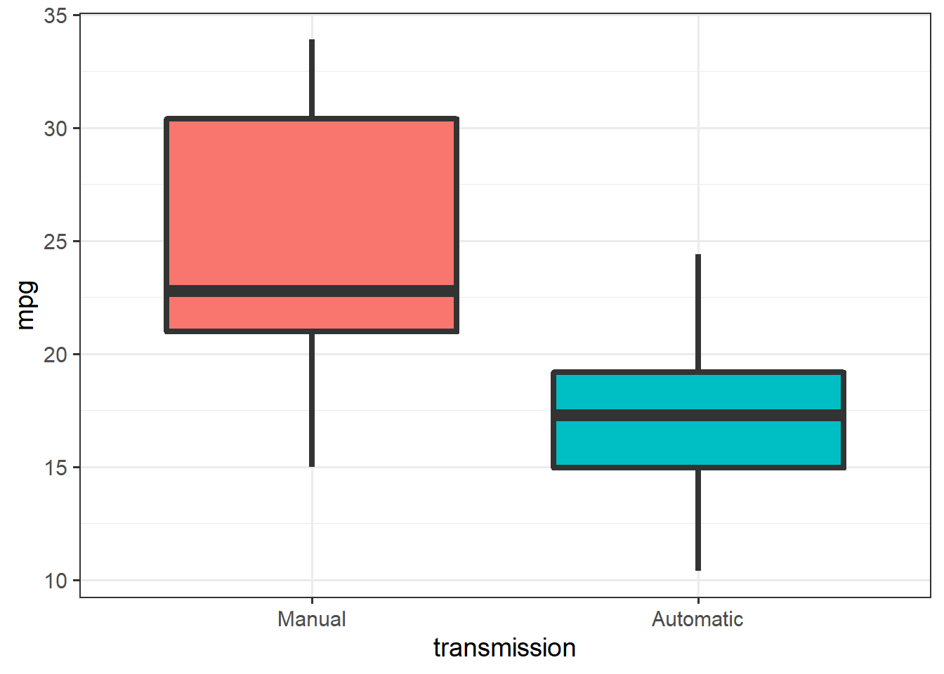
Checking distribution
Before starting any analysis, though, we check the distribution of the response variable:
ggplot(mtcars, aes(x=mpg)) + theme_bw(14)  +
  geom_density(alpha=0.5, fill="lightblue") +
  geom_histogram(aes(y=..density..),
                 binwidth=1, fill="lightgreen",
                 alpha=0.8, colour="black") +
  stat_function(data=mtcars,
                fun = dnorm,
                args=list(mean=mean(mtcars$mpg),
                          sd=sd(mtcars$mpg)),
                colour="blue",
                size=1.1) +
   xlim(c(0,40))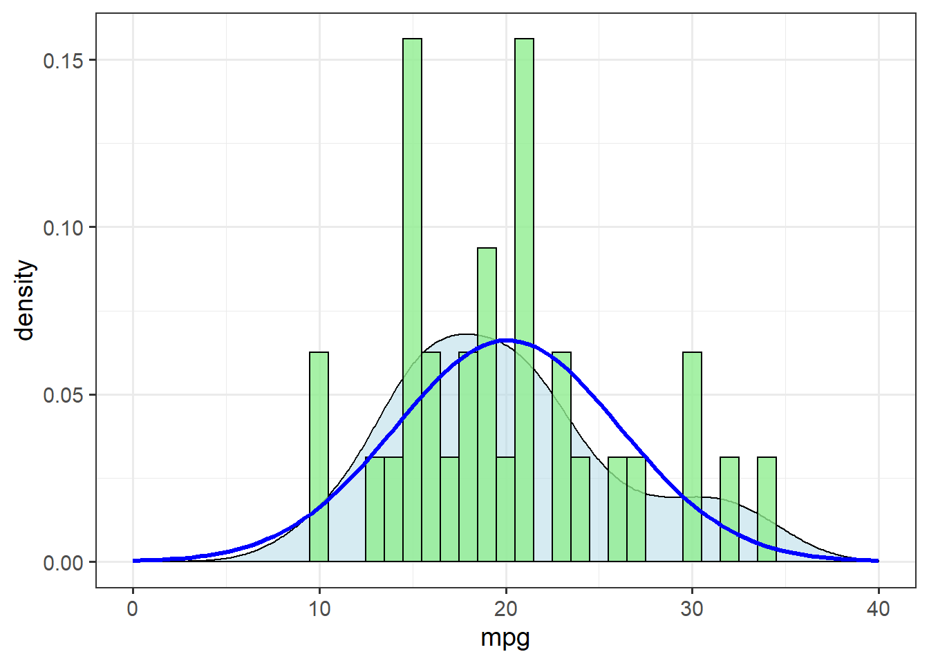
The theoretical distribution (blue line) doesn’t match up terribly well with the density estimate (shaded area). Let’s check for skewness by calculating the ratio of the mean and median:
tibble(Mean = mean(mtcars$mpg),
       Median = median(mtcars$mpg),
       Ratio = Mean/Median)  %>%
 mutate_all(~round(.,2)) %>%
knitr::kable( )| Mean | Median | Ratio |
|---|---|---|
| 20.09 | 19.2 | 1.05 |
Indeed, there is marginal evidence for a right skew in these data. Let’s check what happens when we apply a log-normal transformation:
tibble(Mean = mean(log(mtcars$mpg)),
       Median = median(log(mtcars$mpg)),
       Ratio = Mean/Median) %>%
  mutate_all(~round(.,2)) %>%
knitr::kable( )| Mean | Median | Ratio |
|---|---|---|
| 2.96 | 2.95 | 1 |
mtcars <- mutate(mtcars, lmpg = log(mpg))

 ggplot(mtcars, aes(x=lmpg)) + theme_bw(14) +
    geom_density(alpha=.5, fill="lightblue") +
    geom_histogram(aes(y=..density..),
                   binwidth=0.1,
                   fill="lightgreen",
                   alpha=0.8,
                   colour="black")  +
  stat_function(data=mtcars,
                fun = dnorm,
                args=list(mean=mean(mtcars$lmpg),
                          sd=sd(mtcars$lmpg)),
                colour="blue",
                size=1.1) +
   xlim(c(2,4))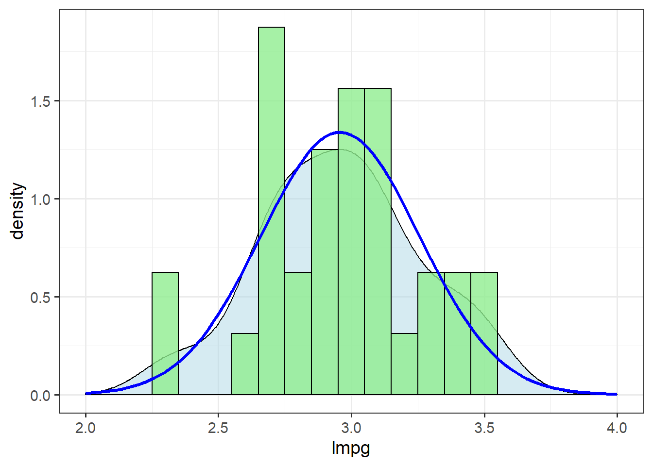
The log-normal transformation improves the fit of these data to the normal distribution.
We’ll use this new column, lmpg, from here on.
t-tests
What does the \(t\)-test actually compare?
Obtain paramaters:
mtcars %>%
group_by(transmission) %>%
  summarize(Mean = mean(lmpg),
            SD = sd(lmpg)) %>%
    mutate_at(vars(Mean, SD), ~round(., 1)) %>%
knitr::kable()| transmission | Mean | SD |
|---|---|---|
| Manual | 3.2 | 0.3 |
| Automatic | 2.8 | 0.2 |
ggplot(mtcars, aes(x=lmpg,
                    fill = transmission)) + theme_bw(14) +
    geom_density(alpha=.5) +
    geom_histogram(aes(y=..density..),
                   binwidth = 0.025,
                   alpha=0.8,
                   colour="black") +
  stat_function(data=mtcars,
                fun = dnorm,
                args=list(mean=2.8,
                          sd=0.2),
                colour="darkred",
                size=2)  +
  stat_function(data=mtcars,
                fun = dnorm,
                args=list(mean = 3.2,
                          sd = 0.3),
                colour="blue",
                size=2)  +
  annotate("label",
           x=c(2.75, 3.25), y=c(1,2),
           label = c("Automatic", "Manual"),
           color=c("darkred", "blue"),
           size=5)
Note that stat_function doesn’t use aes() so can’t map by a variable. Splitting a stat_function by a variable in one plot requires calling stat_function for each factor level.
Testing for differences in groups with a \(t\)-test basically means trying to determine whether the means are really that different based on the spread around them (measured as the standard deviation).
It is straightforward to calculate a \(t\)-statistic. It is simply a ratio of the difference between the means and the variance. This equation is for a variant of the \(t\) test called Welch’s two-sample \(t\) test, which accommodates differences in \(sd\) and \(n\) across the groups:
\(t_{welch} = \frac{\bar{X}_1 - \bar{X}_2}{\sqrt{\frac{s^2_1}{n_1}+\frac{s^2_2}{n_2}}}\)
where \(\bar{X}_1\) and \(\bar{X}_2\) are the means of the two groups (Automatic and Manual transmissions), and \(s\) & \(n\) are the standard deviations and sample sizes, respectively, of each group.
We can define these variables as objects:
mtcars %>%
group_by(transmission) %>%
  summarize(Mean = mean(lmpg),
            SD = sd(lmpg),
            n = n()) %>%
    mutate_at(vars(Mean, SD), ~round(., 3)) %>%
knitr::kable()| transmission | Mean | SD | n |
|---|---|---|---|
| Manual | 3.163 | 0.263 | 13 |
| Automatic | 2.817 | 0.235 | 19 |
# Group means
  X_a = 2.817
  X_m = 3.163
# Standard deviations
  s_a = 0.235
  s_m = 0.263
# Sample sizes
  n_a = 19
  n_m = 13

t_w = (X_m - X_a) / sqrt((s_m^2/n_m) + (s_a^2/n_a) )
t_w
## [1] 3.814593This value indicates that cars with manual transmissions tend to have better fuel economy than those with automatic transmissions. The absolute value of the t statistic is a measure of the size of the difference.
To determine if the effect calculated here is statistically significant, though, the \(t\) value must be compared against a t distribution based on the statistical power of the test (sample size \(n\)).
We’re going to skip this calculation and use the convenient t.test() function to perform the whole test for us:
t.test(lmpg ~ transmission, mtcars)##
## Welch Two Sample t-test
##
## data: lmpg by transmission
## t = 3.8257, df = 23.958, p-value = 0.0008194
## alternative hypothesis: true difference in means is not equal to 0
## 95 percent confidence interval:
## 0.1596180 0.5336626
## sample estimates:
## mean in group Manual mean in group Automatic
## 3.163332 2.816692We see a similar t statistic (slightly different because of our rounding).
Although the overall sample size is 32 and degrees of freedom is \(n-2\), the Welch’s df is lower because the model slightly penalizes the unequal variance.1
But the \(P\) value is well below 0.05, the generally-accepted threshold for statistical significance in the natural sciences.
Furthermore, the 95% confidence interval does not include zero, which would indicate no effect.
Thus, we conclude that yes, there is strong statistical evidence that cars with manual transmissions have better fuel economy than those with automatic transmissions.
Analysis of variance
The \(t\) test is a good illustration of the basic approach behind statistics – comparing the ratio of the difference in the means against the variance – but one rarely uses it, if ever. More often one uses analysis of variance, or ANOVA, to compare differences between two or more groups (the main limitation of \(t\)-tests is that they just compare two groups at a time).
Because ANOVA is a special case of linear regression, the workhorse function for fitting linear models in \({\bf\textsf{R}}\) is lm():
tr_lm <- lm(lmpg ~ transmission, mtcars)We have several options to assess the results of the test, which is stored as an object of class lm.
Simply calling the object reminds us what variables and data we used and the coefficients:
tr_lm##
## Call:
## lm(formula = lmpg ~ transmission, data = mtcars)
##
## Coefficients:
## (Intercept) transmissionAutomatic
## 3.1633 -0.3466The coefficients refer to the essential terms used to describe a line, the intercept \(\beta_0\) and the slope \(\beta_1\):
\(y_i = \beta_0 + \beta_1 x_i + \varepsilon\)
Like the \(t\) statistic, the coefficients give us a measure of the magnitude of the difference between the fule economy of cars with automatic transmissions (transmissionAutomatic) and manual transmissions, which is actually stored here as the Intercept.
So the coefficient of the transmission term is the difference between the group means:
X_a - X_m## [1] -0.346is the same as transmissionManual
coef(tr_lm)## (Intercept) transmissionAutomatic
## 3.1633321 -0.3466403summary() and anova() are two ways to view results of statistical tests in the lm object.
summary() summarizes the linear model fit, giving coefficient estimates, \(t\) statistics, and \(P\) values.
It also returns \(R^2\) values and a summary of an \(F\) test:
summary(tr_lm)##
## Call:
## lm(formula = lmpg ~ transmission, data = mtcars)
##
## Residuals:
## Min 1Q Median 3Q Max
## -0.4749 -0.1213 0.0073 0.1693 0.3779
##
## Coefficients:
## Estimate Std. Error t value Pr(>|t|)
## (Intercept) 3.16333 0.06834 46.290 < 2e-16 ***
## transmissionAutomatic -0.34664 0.08869 -3.909 0.000491 ***
## ---
## Signif. codes: 0 '***' 0.001 '**' 0.01 '*' 0.05 '.' 0.1 ' ' 1
##
## Residual standard error: 0.2464 on 30 degrees of freedom
## Multiple R-squared: 0.3374, Adjusted R-squared: 0.3153
## F-statistic: 15.28 on 1 and 30 DF, p-value: 0.0004905anova() returns the full ANOVA table from the \(F\) test (by default):
anova(tr_lm)## Analysis of Variance Table
##
## Response: lmpg
## Df Sum Sq Mean Sq F value Pr(>F)
## transmission 1 0.92748 0.92748 15.278 0.0004905 ***
## Residuals 30 1.82126 0.06071
## ---
## Signif. codes: 0 '***' 0.001 '**' 0.01 '*' 0.05 '.' 0.1 ' ' 1Remember, this is Intro to \({\bf\textsf{R}}\), not intro to statistics, so we aren’t going to dig into where these values come from or the differences between the linear model fit and the \(F\) test, just how to get them with \({\bf\textsf{R}}\). If the statistical terms here are unfamiliar to you, or if you need to brush up, I recommend going through another post, How ANOVA is linear regression.
Multiple comparisons
The difference between summary(), which returns \(t\) statistics, and anova(), which returns \(F\) statistics, becomes complicated for models with three or more groups:
ggplot(mtcars, aes(x=cyl, y=mpg)) + theme_bw(14) +
geom_boxplot(aes(fill=cyl), show.legend = F) 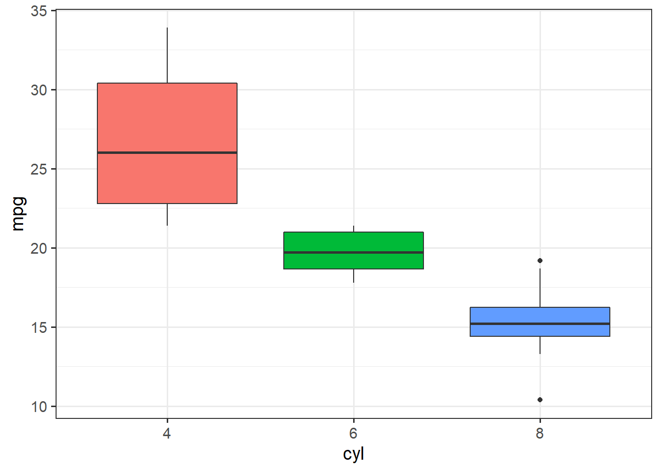
# Fit a model:
  cyl_lm <- lm(mpg ~ cyl, mtcars)
And compare the results:
anova(cyl_lm)## Analysis of Variance Table
##
## Response: mpg
## Df Sum Sq Mean Sq F value Pr(>F)
## cyl 2 824.78 412.39 39.697 4.979e-09 ***
## Residuals 29 301.26 10.39
## ---
## Signif. codes: 0 '***' 0.001 '**' 0.01 '*' 0.05 '.' 0.1 ' ' 1summary(cyl_lm)##
## Call:
## lm(formula = mpg ~ cyl, data = mtcars)
##
## Residuals:
## Min 1Q Median 3Q Max
## -5.2636 -1.8357 0.0286 1.3893 7.2364
##
## Coefficients:
## Estimate Std. Error t value Pr(>|t|)
## (Intercept) 26.6636 0.9718 27.437 < 2e-16 ***
## cyl6 -6.9208 1.5583 -4.441 0.000119 ***
## cyl8 -11.5636 1.2986 -8.905 8.57e-10 ***
## ---
## Signif. codes: 0 '***' 0.001 '**' 0.01 '*' 0.05 '.' 0.1 ' ' 1
##
## Residual standard error: 3.223 on 29 degrees of freedom
## Multiple R-squared: 0.7325, Adjusted R-squared: 0.714
## F-statistic: 39.7 on 2 and 29 DF, p-value: 4.979e-09The ANOVA table has a single term for cyl, and gives a positive \(F\) statistic because the \(F\) distribution is one-sided.
The linear model results, though, are more complete, with two terms for each of the groups beyond 4 cylinder cars.
The results show that both 6 cylinder engines and 8 cylinder engines get significantly lower fuel economy than 4 cylinder engines, but the test does not compare 6 vs. 8 cylinder engines.
The solution is post-hoc pairwise comparisons of all group comparisons within the cyl term in the ANOVA model, for which \({\bf\textsf{R}}\) provides the TukeyHSD() function (“Tukey’s Honest Significant Differences”).
But we first need to explicitly convert the lm object to an ANOVA model with aov():2
aov(cyl_lm) %>% TukeyHSD() ## Tukey multiple comparisons of means
## 95% family-wise confidence level
##
## Fit: aov(formula = cyl_lm)
##
## $cyl
## diff lwr upr p adj
## 6-4 -6.920779 -10.769350 -3.0722086 0.0003424
## 8-4 -11.563636 -14.770779 -8.3564942 0.0000000
## 8-6 -4.642857 -8.327583 -0.9581313 0.0112287These results confirm that in all combinations, group means are significantly different from each other.
The Tukey method adjusts the \(P\) values to account for multiple comparisons in one model, making this a robust approach to running several independent pairwise tests.