This post illustrates how Analysis of Variance – ANOVA, used for testing for differences among groups – is a special case of linear regression.
Along the way, we parse the various components of results from statistical tests in \({\bf\textsf{R}}\) and illustrate post-hoc pairwise tests using TukeyHSD().
The statistics of a line
Recall that the arithmetic equation for a line, y = mx + b, is expressed statistically as
\(y_i = \beta_0 + \beta_1 x_i + \varepsilon\)
in which \(\beta_0\) is where the line crosses the Y axis (intercept), \(\beta_1\) is the slope of the line, and \(\varepsilon\) is the residual error that remains unexplained by the linear relationship between \(x\) and \(y\).
In linear regression, we are often most interested in the slope, \(\beta_1\). This is where the action is, the measure of the strength of the effect we are testing for.
In terms of hypotheses, consider the null, \(H_0\), versus an alternative hypothesis, \(H_1\), about the relationship between two variables, X and Y:
\(H_0\): No effect. The value of Y has no discernable pattern in response to changes in the value of X.
\(H_1\): The value of Y changes right along with changes in X.
Linear regression on continuous data
There are various ways to draw \(H_0\), but let’s focus on what it means in terms of the slope of a line. If slope is a measure of effect and there is zero effect, we’d expect zero slope, as well, or \(\beta_1 = 0\):
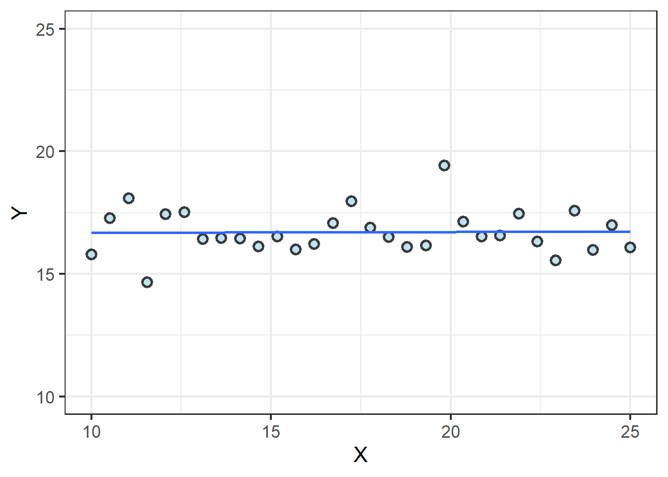
We can use lm() to estimate the two parts of this line, the intercept \(\beta_0\), and the slope, \(\beta_0\):
m1 <- lm(Y ~ X, line_data)
coef(m1)
## (Intercept) X
## 16.648587544 0.003142142As is clear from the graph, the line crosses the Y axis at 16.6 and has a slope dang near 0. We have no evidence on which to reject the null hypothesis.
Now consider a case in which the value of Y quite clearly increases with the value of X:

m2 <- lm(Y ~ X, line_data)
coef(m2)
## (Intercept) X
## -47.038254 5.089453This line crosses the Y axis at -47 and for every 1 unit X increases, Y increases 5 units. Hence, as X goes from 15 to 20, Y increases \(5~\times~5\) units, from 30 to 55. This is likely enough evidence to reject the null hypothesis, and the \(P\) value confirms it:
summary(m2)$coefficients| .rownames | Estimate | Std..Error | t.value | Pr…t.. |
|---|---|---|---|---|
| (Intercept) | -47.04 | 11.38 | -4.133 | 0.0002942 |
| X | 5.089 | 0.6301 | 8.077 | 8.553e-09 |
Both the intercept and slope are significantly different from 0, based on the \(t\) statistic for each term, with \(P\) values derived from the \(t\) distribution based on the model’s degrees of freedom. As with even a basic \(t\)-test, the \(t\) statistic in the summary table of the linear model is calculated as the ratio of the estimated effect (the coefficient) and the error around that estimate:
# Intercept (Beta 0)
  -47.04 / 11.38
## [1] -4.133568# X (Beta 1)
5.089 / 0.6301## [1] 8.076496Fitting lines to categorical data
It makes sense to apply linear regression on continuous data – we have a cloud of points through which we can try to draw a line that minimizes the distance between each point and the line.
It can be less intuitive how we can approach categorical data, which appear as distinct clusters…

… until we focus on the fact that linear regression on continuous data begins with treating them as a single cluster.
Wait, what? It is true. While it might be tempting to think of the regression line spurting out from the Y axis at the intercept or something, every regression line actually begins at the same point: where the means of the X and Y values intersect:
| Mean of X | Mean of Y |
|---|---|
| 17.5 | 42.03 |
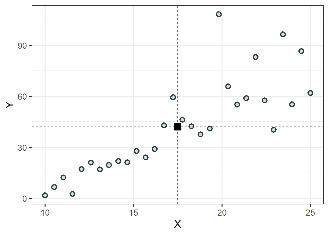
The regression equation then finds the slope of a line that minimizes the distance between the line and each observation. Because half of the points will fall below the line and the other half above, the distances between each point and the line are squared to ensure their absolute value, otherwise the total error would be zero, with half of the values being negative! It is this process of minimizing the squared error between all points and the regression line that gives us the term least squares regression. Only once the slope of this line is calculated is the point where the line crosses the Y axis determined.
Comparing two groups
It becomes easy, then, to imagine finding the group means in the categorical data (let’s start with just two groups):
| Group | Group mean |
|---|---|
| A | 13.85 |
| B | 6.78 |

We know the old saying, two points make a line, and here we have two points… so let’s connect them with a line:
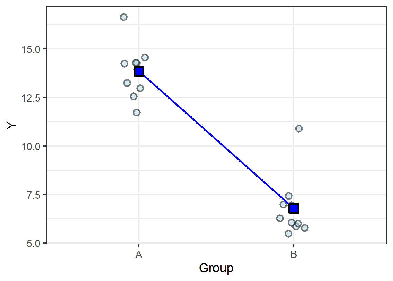
From here it is easy to see how a slope can be calculated from the difference between the means.
But slope (\(\beta_1\)) is just one of the two terms required to statistically describe a line. We also need an intercept (\(\beta_0\)).
This is the genius of ANOVA – how it gets an intercept from two categorical variables. It does so by simply assigning the first group to X = 0, making its mean by default the Y intercept. The next group is tested as X = 1, so the difference in the means is by default the slope, because when \(\Delta X = 1\),
\(\frac{\Delta Y}{\Delta X} = \frac{\Delta Y}{1} = \Delta Y\):
m3 <- lm(Y ~ Group, group_data)
coef(m3)| Term | Coefficient |
|---|---|
| (Intercept) | 13.85 |
| GroupB | -7.07 |
Indeed, \(\beta_0 = 13.85\), and \(\beta_1 = -7.07\), because \(13.85 - 6.78 = 7.07\)
summary(m3)$coefficients %>%
pander::pander() | Estimate | Std. Error | t value | Pr(>|t|) | |
|---|---|---|---|---|
| (Intercept) | 13.85 | 0.4625 | 29.95 | 8.262e-17 |
| GroupB | -7.07 | 0.654 | -10.81 | 2.658e-09 |
Again, the model tells us whether the difference between the means is significant relative to the variance by calculating a \(t\) statistic and finding its P value from the t distribution based on the degrees of freedom.
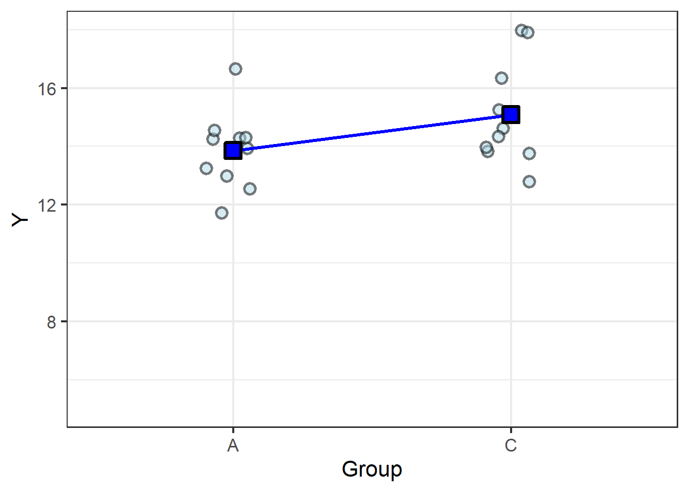
To round out the example, let’s consider a case in which there is no difference between the means:
| Group | Group mean |
|---|---|
| A | 13.85 |
| C | 15.08 |
m4 <- lm(Y ~ Group, filter(group_data, Group !="B"))
summary(m4)$coefficients %>%
pander::pander() | Estimate | Std. Error | t value | Pr(>|t|) | |
|---|---|---|---|---|
| (Intercept) | 13.85 | 0.4982 | 27.8 | 3.069e-16 |
| GroupC | 1.231 | 0.7046 | 1.747 | 0.09764 |
The difference in the means, \(1.2\), isn’t substantially greater than the variance, \(0.7\), so the resulting \(t\) statistic, \(1.7\), is too small to return a \(P\) value below the generally-accepted \(P = 0.05\). Thus the model confirms what we can see from the graph: the slope is too shallow, meaning there’s no meaningful difference between the group means.
t-statistics vs. F statistics
So far we’ve focused on the \(t\) statistic, which is returned by calls to summary() on lm objects.
\(t\) statistics are useful because the \(t\) distribution is two-sided and symetrical, like a normal distribution.
Thus, \(t\) values can either be negative or positive: the sign corresponds to the direction of the effect (increasing or decreasing), and the absolute value measures the size of the effect.
An alternative to the \(t\) statistic is the \(F\) statistic, which is based on a one-sided \(F\) distribution and is returned by an \(F\) test.
The results of the \(F\) test are returned at the end of the results of summary():
summary(m3)##
## Call:
## lm(formula = Y ~ Group, data = filter(group_data, Group != "C"))
##
## Residuals:
## Min 1Q Median 3Q Max
## -2.1208 -0.8761 -0.2030 0.4395 4.1186
##
## Coefficients:
## Estimate Std. Error t value Pr(>|t|)
## (Intercept) 13.8507 0.4625 29.95 < 2e-16 ***
## GroupB -7.0703 0.6540 -10.81 2.66e-09 ***
## ---
## Signif. codes: 0 '***' 0.001 '**' 0.01 '*' 0.05 '.' 0.1 ' ' 1
##
## Residual standard error: 1.462 on 18 degrees of freedom
## Multiple R-squared: 0.8665, Adjusted R-squared: 0.8591
## F-statistic: 116.9 on 1 and 18 DF, p-value: 2.658e-09We can also perform the \(F\) test alone – and get a full ANOVA table – by calling anova() on the lm object:
anova(m3) | term | df | sumsq | meansq | statistic | p.value |
|---|---|---|---|---|---|
| Group | 1 | 249.9 | 249.9 | 116.9 | 2.658e-09 |
| Residuals | 18 | 38.5 | 2.139 | NA | NA |
Yet again, the \(F\) statistic is obtained by comparing the term we hypothesize explains variation in the response variable (Group) against the error that remains unexplained (Residuals):
\(F = \frac{Mean~Sum~Squares_{Group}}{Mean~Sum~Squares_{Residuals}}\)
\(116.9 = \frac{249.9}{2.139}\)
The \(F\) test indicates that this is a statistically-significant effect, but because the \(F\) distribution is one-sided, we do not know whether the effect was an increase or a decrease without seeing the data or knowing the group means.
Comparing three (or more) groups
The \(F\) test is unique because it conducts a “global” test of the independent cateogrical variable. Compare the results of tests of Groups B and C against A:
| term | df | sumsq | meansq | statistic | p.value |
|---|---|---|---|---|---|
| Group | 1 | 249.9 | 249.9 | 116.9 | 2.658e-09 |
| Residuals | 18 | 38.5 | 2.139 | NA | NA |
| term | df | sumsq | meansq | statistic | p.value |
|---|---|---|---|---|---|
| Group | 1 | 7.577 | 7.577 | 3.053 | 0.09764 |
| Residuals | 18 | 44.68 | 2.482 | NA | NA |
But unlike a basic pairwise \(t\)-test, we can also test all three groups together:
m_all <- lm(Y ~ Group, group_data)
anova(m_all)| term | df | sumsq | meansq | statistic | p.value |
|---|---|---|---|---|---|
| Group | 2 | 401.39 | 200.69 | 80.9 | 0 |
| Residuals | 27 | 66.98 | 2.48 | NA | NA |
This is confusing, because the model returns a significant P value even though we know that one combination of means are not different (A vs. C).
When there are three or more groups in an \(F\) test, we must interpret a significant result as telling us that at least one group mean is different from at least one other group mean. Every group mean could be different from every other group mean, or only a single combination is different, or any combination in between. We just don’t know from the basic output of the \(F\) test. This is a second limitation (in addition to the one-sided \(F\) statistic).
Post-hoc Tukey tests
The output of the linear regression model provides insight into group-group comparisons:
summary(m_all)| term | estimate | std.error | statistic | p.value |
|---|---|---|---|---|
| (Intercept) | 13.85 | 0.5 | 27.81 | 0.00 |
| GroupB | -7.07 | 0.7 | -10.04 | 0.00 |
| GroupC | 1.23 | 0.7 | 1.75 | 0.09 |
This table combines the results of the pairwise tests we conducted above: \(\beta_0\) is the mean of Group A, and estimates for Group B and Group C (\(\beta_{1~(aka~A-B)}\) and \(\beta_{2~(aka~A-C)}\), respectively) appear as the difference from Group A.
It should be clear that the additional terms, \(\beta_{1~(aka~A-B)}\) and \(\beta_{2~(aka~A-C)}\), are tested against the intercept, \(\beta_{0~(aka~A)}\). But what about the relationship between Group B and Group C? We do not get a t statistic for this comparison.
The solution is what is called post-hoc pairwise comparisons.
A popular option is the post-hoc Tukey test, aka “Tukey’s Honest Significant Differences”, which informs the \({\bf\textsf{R}}\) function TukeyHSD().
Unfortunately, TukeyHSD() will not work on an lm object, so we convert it with the aov() function first:
aov(m_all) %>% TukeyHSD()| comparison | estimate | conf.low | conf.high | adj.p.value |
|---|---|---|---|---|
| B-A | -7.07 | -8.82 | -5.32 | 0.00 |
| C-A | 1.23 | -0.52 | 2.98 | 0.21 |
| C-B | 8.30 | 6.55 | 10.05 | 0.00 |
These are very informative results. The table gives us directions for each estimate, which corresponds to the magnitude of the effect for each pairwise comparison. We also get a 95% confidence interval around the estimate, as a measure of precision. The resulting p values have been adjusted to correct for the fact that multiple comparisons are being made simultaneously; this is a robust feature that makes the post-hoc test both an elegant and statistically-valid alternative to conducting separate t-tests among each combination of groups.